Lab 1: MC Statistical Analysis
Topics covered in this lab
This lab focuses on the basics of analyzing data from MC calculations. In this lab, participants will use data from VMC calculations of a simple 1-electron system with an analytically soluble system (the ground state of the hydrogen atom) to understand how to interpret an MC situation. Most of these analyses will also carry over to DMC simulations. Topics covered include:
Averaging MC variables
The statisical error bar of mean values
The effects of autocorrelation and variance on the error bar
The relationship between MC time step and autocorrelation
The use of blocking to reduce autocorrelation
The significance of the acceptance ratio
The significance of the sample size
How to determine whether an MC run was successful
The relationship between wavefunction quality and variance
Gauging the efficiency of MC runs
The cost of scaling up to larger system sizes
Lab directories and files
labs/lab1_qmc_statistics/
│
├── atom                              - H atom VMC calculation
│   ├── H.s000.scalar.dat                - H atom VMC data
│   └── H.xml                            - H atom VMC input file
│
├── autocorrelation                   - varying autocorrelation
│   ├── H.dat                            - data for gnuplot
│   ├── H.plt                            - gnuplot for time step vs. E_L, tau_c
│   ├── H.s000.scalar.dat                - H atom VMC data: time step = 10
│   ├── H.s001.scalar.dat                - H atom VMC data: time step =  5
│   ├── H.s002.scalar.dat                - H atom VMC data: time step =  2
│   ├── H.s003.scalar.dat                - H atom VMC data: time step =  1
│   ├── H.s004.scalar.dat                - H atom VMC data: time step =  0.5
│   ├── H.s005.scalar.dat                - H atom VMC data: time step =  0.2
│   ├── H.s006.scalar.dat                - H atom VMC data: time step =  0.1
│   ├── H.s007.scalar.dat                - H atom VMC data: time step =  0.05
│   ├── H.s008.scalar.dat                - H atom VMC data: time step =  0.02
│   ├── H.s009.scalar.dat                - H atom VMC data: time step =  0.01
│   ├── H.s010.scalar.dat                - H atom VMC data: time step =  0.005
│   ├── H.s011.scalar.dat                - H atom VMC data: time step =  0.002
│   ├── H.s012.scalar.dat                - H atom VMC data: time step =  0.001
│   ├── H.s013.scalar.dat                - H atom VMC data: time step =  0.0005
│   ├── H.s014.scalar.dat                - H atom VMC data: time step =  0.0002
│   ├── H.s015.scalar.dat                - H atom VMC data: time step =  0.0001
│   └── H.xml                            - H atom VMC input file
│
├── average                            - Python scripts for average/std. dev.
│   ├── average.py                         - average five E_L from H atom VMC
│   ├── stddev2.py                         - standard deviation using (E_L)^2
│   └── stddev.py                          - standard deviation around the mean
│
├── basis                              - varying basis set for orbitals
│   ├── H__exact.s000.scalar.dat           - H atom VMC data using STO basis
│   ├── H_STO-2G.s000.scalar.dat           - H atom VMC data using STO-2G basis
│   ├── H_STO-3G.s000.scalar.dat           - H atom VMC data using STO-3G basis
│   └── H_STO-6G.s000.scalar.dat           - H atom VMC data using STO-6G basis
│
├── blocking                           - varying block/step ratio
│   ├── H.dat                              - data for gnuplot
│   ├── H.plt                              - gnuplot for N_block vs. E, tau_c
│   ├── H.s000.scalar.dat                  - H atom VMC data 50000:1 blocks:steps
│   ├── H.s001.scalar.dat                  - "  "    "    "  25000:2 blocks:steps
│   ├── H.s002.scalar.dat                  - "  "    "    "  12500:4 blocks:steps
│   ├── H.s003.scalar.dat                  - "  "    "    "  6250: 8 blocks:steps
│   ├── H.s004.scalar.dat                  - "  "    "    "  3125:16 blocks:steps
│   ├── H.s005.scalar.dat                  - "  "    "    "  2500:20 blocks:steps
│   ├── H.s006.scalar.dat                  - "  "    "    "  1250:40 blocks:steps
│   ├── H.s007.scalar.dat                  - "  "    "    "  1000:50 blocks:steps
│   ├── H.s008.scalar.dat                  - "  "    "    "  500:100 blocks:steps
│   ├── H.s009.scalar.dat                  - "  "    "    "  250:200 blocks:steps
│   ├── H.s010.scalar.dat                  - "  "    "    "  125:400 blocks:steps
│   ├── H.s011.scalar.dat                  - "  "    "    "  100:500 blocks:steps
│   ├── H.s012.scalar.dat                  - "  "    "    "  50:1000 blocks:steps
│   ├── H.s013.scalar.dat                  - "  "    "    "  40:1250 blocks:steps
│   ├── H.s014.scalar.dat                  - "  "    "    "  20:2500 blocks:steps
│   ├── H.s015.scalar.dat                  - "  "    "    "  10:5000 blocks:steps
│   └── H.xml                             - H atom VMC input file
│
├── blocks                             -  varying total number of blocks
│   ├── H.dat                             - data for gnuplot
│   ├── H.plt                             - gnuplot for N_block vs. E
│   ├── H.s000.scalar.dat                 - H atom VMC data    500 blocks
│   ├── H.s001.scalar.dat                 - "  "    "    "    2000 blocks
│   ├── H.s002.scalar.dat                 - "  "    "    "    8000 blocks
│   ├── H.s003.scalar.dat                 - "  "    "    "   32000 blocks
│   ├── H.s004.scalar.dat                 - "  "    "    "  128000 blocks
│   └── H.xml                             - H atom VMC input file
│
├── dimer                          - comparing no and simple Jastrow factor
│   ├── H2_STO___no_jastrow.s000.scalar.dat - H dimer VMC data without Jastrow
│   └── H2_STO_with_jastrow.s000.scalar.dat - H dimer VMC data with Jastrow
│
├──  docs                               - documentation
│   ├──  Lab_1_MC_Analysis.pdf             - this document
│   └──  Lab_1_Slides.pdf                  - slides presented in the lab
│
├── nodes                              - varying number of computing nodes
│   ├──  H.dat                             - data for gnuplot
│   ├──  H.plt                             - gnuplot for N_node vs. E
│   ├──  H.s000.scalar.dat                 - H atom VMC data with  32 nodes
│   ├──  H.s001.scalar.dat                 - H atom VMC data with 128 nodes
│   └──  H.s002.scalar.dat                 - H atom VMC data with 512 nodes
│
├── problematic                        - problematic VMC run
│   └──  H.s000.scalar.dat                 - H atom VMC data with a problem
│
└── size                                - scaling with number of particles
    ├──  01________H.s000.scalar.dat       - H atom VMC data
    ├──  02_______H2.s000.scalar.dat       - H dimer "   "
    ├──  06________C.s000.scalar.dat       - C atom  "   "
    ├──  10______CH4.s000.scalar.dat       - methane "   "
    ├──  12_______C2.s000.scalar.dat       - C dimer "   "
    ├──  16_____C2H4.s000.scalar.dat       - ethene  "
    ├──  18___CH4CH4.s000.scalar.dat       - methane dimer VMC data
    ├──  32_C2H4C2H4.s000.scalar.dat       - ethene dimer   "   "
    ├──  nelectron_tcpu.dat                - data for gnuplot
    └──  Nelectron_tCPU.plt                - gnuplot for N_elec vs. t_CPU
Atomic units
QMCPACK operates in Ha atomic units to reduce the number of factors in the Schrödinger equation. Thus, the unit of length is the bohr (5.291772 \(\times 10^{-11}\) m = 0.529177 Å); the unit of energy is the Ha (4.359744 \(\times 10^{-18}\) J = 27.211385 eV). The energy of the ground state of the hydrogen atom in these units is -0.5 Ha.
Reviewing statistics
We will practice taking the average (mean) and standard deviation of some MC data by hand to review the basic definitions.
Enter Python’s command line by typing python [Enter]. You will see a
prompt “>>>.”
The mean of a dataset is given by:
To calculate the average of five local energies from an MC calculation
of the ground state of an electron in the hydrogen atom, input (truncate
at the thousandths place if you cannot copy and paste; script versions
are also available in the average directory):
(
(-0.45298911858) +
(-0.45481953564) +
(-0.48066105923) +
(-0.47316713469) +
(-0.46204733302)
)/5.
Then, press [Enter] to get:
>>> ((-0.45298911858) + (-0.45481953564) + (-0.48066105923) +
(-0.47316713469) + (-0.4620473302))/5.
-0.46473683566800006
To understand the significance of the mean, we also need the standard deviation around the mean of the data (also called the error bar), given by:
To calculate the standard deviation around the mean (-0.464736835668) of these five data points, put in:
( (1./(5.*(5.-1.))) * (
(-0.45298911858-(-0.464736835668))**2 + \\
(-0.45481953564-(-0.464736835668))**2 +
(-0.48066105923-(-0.464736835668))**2 +
(-0.47316713469-(-0.464736835668))**2 +
(-0.46204733302-(-0.464736835668))**2 )
)**0.5
Then, press [Enter] to get:
>>> ( (1./(5.*(5.-1.))) * ( (-0.45298911858-(-0.464736835668))**2 +
(-0.45481953564-(-0.464736835668))**2 + (-0.48066105923-(-0.464736835668))**2 +
(-0.47316713469-(-0.464736835668))**2 + (-0.46204733302-(-0.464736835668))**2
) )**0.5
0.0053303187464332066
Thus, we might report this data as having a value -0.465 +/- 0.005 Ha. This calculation of the standard deviation assumes that the average for this data is fixed, but we can continually add MC samples to the data, so it is better to use an estimate of the error bar that does not rely on the overall average. Such an estimate is given by:
To calculate the standard deviation with this formula, input the following, which includes the square of the local energy calculated with each corresponding local energy:
( (1./(5.-1.)) * (
(0.60984565298-(-0.45298911858)**2) + \\
(0.61641291630-(-0.45481953564)**2) +
(1.35860151160-(-0.48066105923)**2) + \\
(0.78720769003-(-0.47316713469)**2) +
(0.56393677687-(-0.46204733302)**2) )
)**0.5
and press [Enter] to get:
>>> ((1./(5.-1.))*((0.60984565298-(-0.45298911858)**2)+
(0.61641291630-(-0.45481953564)**2)+(1.35860151160-(-0.48066105923)**2)+
(0.78720769003-(-0.47316713469)**2)+(0.56393677687-(-0.46204733302)**2))
)**0.5
0.84491636672906634
This much larger standard deviation, acknowledging that the mean of this small data set is not the average in the limit of infinite sampling, more accurately reports the value of the local energy as -0.5 +/- 0.8 Ha.
Type quit() and press [Enter] to exit the Python command line.
Inspecting MC Data
QMCPACK outputs data from MC calculations into files ending in
scalar.dat. Several quantities are calculated and written for each
block of MC steps in successive columns to the right of the step index.
Change directories to atom, and open the file ending in
scalar.dat with a text editor (e.g., vi *.scalar.dat or emacs
*.scalar.dat. If possible, adjust the terminal so that lines do not
wrap. The data will begin as follows (broken into three groups to fit on
this page):
#   index    LocalEnergy         LocalEnergy_sq      LocalPotential     ...
         0   -4.5298911858e-01    6.0984565298e-01   -1.1708693521e+00
         1   -4.5481953564e-01    6.1641291630e-01   -1.1863425644e+00
         2   -4.8066105923e-01    1.3586015116e+00   -1.1766446209e+00
         3   -4.7316713469e-01    7.8720769003e-01   -1.1799481122e+00
         4   -4.6204733302e-01    5.6393677687e-01   -1.1619244081e+00
         5   -4.4313854290e-01    6.0831516179e-01   -1.2064503041e+00
         6   -4.5064926960e-01    5.9891422196e-01   -1.1521370176e+00
         7   -4.5687452611e-01    5.8139614676e-01   -1.1423627617e+00
         8   -4.5018503739e-01    8.4147849706e-01   -1.1842075439e+00
         9   -4.3862013841e-01    5.5477715836e-01   -1.2080979177e+00
The first line begins with a #, indicating that this line does not contain MC data but rather the labels of the columns. After a blank line, the remaining lines consist of the MC data. The first column, labeled index, is an integer indicating which block of MC data is on that line. The second column contains the quantity usually of greatest interest from the simulation: the local energy. Since this simulation did not use the exact ground state wavefunction, it does not produce -0.5 Ha as the local energy although the value lies within about 10%. The value of the local energy fluctuates from block to block, and the closer the trial wavefunction is to the ground state the smaller these fluctuations will be. The next column contains an important ingredient in estimating the error in the MC average—the square of the local energy—found by evaluating the square of the Hamiltonian.
...   Kinetic             Coulomb             BlockWeight        ...
       7.1788023352e-01   -1.1708693521e+00    1.2800000000e+04
       7.3152302871e-01   -1.1863425644e+00    1.2800000000e+04
       6.9598356165e-01   -1.1766446209e+00    1.2800000000e+04
       7.0678097751e-01   -1.1799481122e+00    1.2800000000e+04
       6.9987707508e-01   -1.1619244081e+00    1.2800000000e+04
       7.6331176120e-01   -1.2064503041e+00    1.2800000000e+04
       7.0148774798e-01   -1.1521370176e+00    1.2800000000e+04
       6.8548823555e-01   -1.1423627617e+00    1.2800000000e+04
       7.3402250655e-01   -1.1842075439e+00    1.2800000000e+04
       7.6947777925e-01   -1.2080979177e+00    1.2800000000e+04
The fourth column from the left consists of the values of the local potential energy. In this simulation, it is identical to the Coulomb potential (contained in the sixth column) because the one electron in the simulation has only the potential energy coming from its interaction with the nucleus. In many-electron simulations, the local potential energy contains contributions from the electron-electron Coulomb interactions and the nuclear potential or pseudopotential. The fifth column contains the local kinetic energy value for each MC block, obtained from the Laplacian of the wavefunction. The sixth column shows the local Coulomb interaction energy. The seventh column displays the weight each line of data has in the average (the weights are identical in this simulation).
...    BlockCPU            AcceptRatio
       6.0178991748e-03    9.8515625000e-01
       5.8323097461e-03    9.8562500000e-01
       5.8213412744e-03    9.8531250000e-01
       5.8330412549e-03    9.8828125000e-01
       5.8108362256e-03    9.8625000000e-01
       5.8254170264e-03    9.8625000000e-01
       5.8314813086e-03    9.8679687500e-01
       5.8258469971e-03    9.8726562500e-01
       5.8158433545e-03    9.8468750000e-01
       5.7959401123e-03    9.8539062500e-01
The eighth column shows the CPU time (in seconds) to calculate the data in that line. The ninth column from the left contains the acceptance ratio (1 being full acceptance) for MC steps in that line’s data. Other than the block weight, all quantities vary from line to line.
Exit the text editor ([Esc] :q! [Enter] in vi, [Ctrl]-x [Ctrl]-c in emacs).
Averaging quantities in the MC data
QMCPACK includes the qmca Python tool to average quantities in the
scalar.dat file (and also the dmc.dat file of DMC simulations).
Without any flags, qmca will output the average of each column with a
quantity in the scalar.dat file as follows.
Execute qmca by qmca *.scalar.dat, which for this data outputs:
H  series 0
LocalEnergy           =          -0.45446 +/-          0.00057
Variance              =             0.529 +/-            0.018
Kinetic               =            0.7366 +/-           0.0020
LocalPotential        =           -1.1910 +/-           0.0016
Coulomb               =           -1.1910 +/-           0.0016
LocalEnergy_sq        =             0.736 +/-            0.018
BlockWeight           =    12800.00000000 +/-       0.00000000
BlockCPU              =        0.00582002 +/-       0.00000067
AcceptRatio           =          0.985508 +/-         0.000048
Efficiency            =        0.00000000 +/-       0.00000000
After one blank, qmca prints the title of the subsequent data, gleaned
from the data file name. In this case, H.s000.scalar.dat became “H
series 0.” Everything before the first “.s” will be interpreted as
the title, and the number between “.s” and the next “.” will be
interpreted as the series number.
The first column under the title is the name of each quantity qmca averaged. The column to the right of the equal signs contains the average for the quantity of that line, and the column to the right of the plus-slash-minus is the statistical error bar on the quantity. All quantities calculated from MC simulations have and must be reported with a statistical error bar!
Two new quantities not present in the scalar.dat file are computed
by qmca from the data—variance and efficiency. We will look at these
later in this lab.
To view only one value, qmca takes the -q (quantity) flag. For
example, the output of qmca -q LocalEnergy *.scalar.dat in this
directory produces a single line of output:
H series 0 LocalEnergy = -0.454460 +/- 0.000568
Type qmca –help to see the list of all quantities and their
abbreviations.
Evaluating MC simulation quality
There are several aspects of a MC simulation to consider in deciding how well it went. Besides the deviation of the average from an expected value (if there is one), the stability of the simulation in its sampling, the autocorrelation between MC steps, the value of the acceptance ratio (accepted steps over total proposed steps), and the variance in the local energy all indicate the quality of an MC simulation. We will look at these one by one.
Tracing MC quantities
Visualizing the evolution of MC quantities over the course of the simulation by a trace offers a quick picture of whether the random walk had the expected behavior. qmca plots traces with the -t flag.
Type qmca -q e -t H.s000.scalar.dat, which produces a graph of the
trace of the local energy:
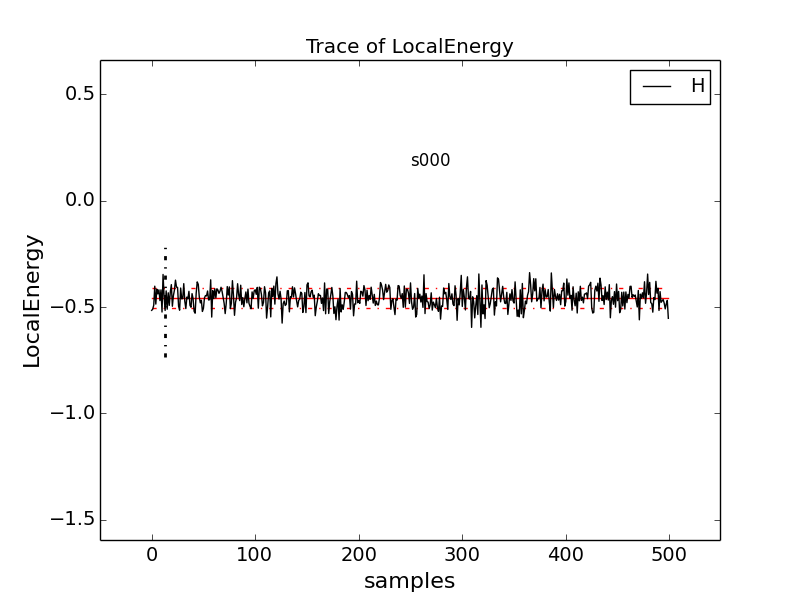
The solid black line connects the values of the local energy at each MC block (labeled “samples”). The average value is marked with a horizontal, solid red line. One standard deviation above and below the average are marked with horizontal, dashed red lines.
The solid black line connects the values of the local energy at each MC block (labeled “samples”). The average value is marked with a horizontal, solid red line. One standard deviation above and below the average are marked with horizontal, dashed red lines.
The trace of this run is largely centered on the average with no large-scale oscillations or major shifts, indicating a good-quality MC run.
Try tracing the kinetic and potential energies, seeing that their behavior is comparable with the total local energy.
Change to directory problematic and type
qmca -q e -t H.s000.scalar.dat to produce this graph:
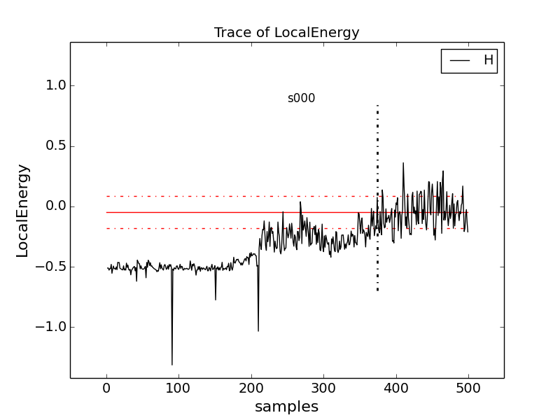
Here, the local energy samples cluster around the expected -0.5 Ha for the first 150 samples or so and then begin to oscillate more wildly and increase erratically toward 0, indicating a poor-quality MC run.
Again, trace the kinetic and potential energies in this run and see how their behavior compares with the total local energy.
Blocking away autocorrelation
Autocorrelation occurs when a given MC step biases subsequent MC steps, leading to samples that are not statistically independent. We must take this autocorrelation into account to obtain accurate statistics. qmca outputs autocorrelation when given the –sac flag.
Change to directory autocorrelation and type
qmca -q e --sac H.s000.scalar.dat.
H series 0 LocalEnergy = -0.454982 +/- 0.000430 1.0
The value after the error bar on the quantity is the autocorrelation (1.0 in this case).
Proposing too small a step in configuration space, the MC time step,
can lead to autocorrelation since the new samples will be in the
neighborhood of previous samples. Type grep timestep H.xml to see
the varying time step values in this QMCPACK input file (H.xml):
<parameter name="timestep">10</parameter>
<parameter name="timestep">5</parameter>
<parameter name="timestep">2</parameter>
<parameter name="timestep">1</parameter>
<parameter name="timestep">0.5</parameter>
<parameter name="timestep">0.2</parameter>
<parameter name="timestep">0.1</parameter>
<parameter name="timestep">0.05</parameter>
<parameter name="timestep">0.02</parameter>
<parameter name="timestep">0.01</parameter>
<parameter name="timestep">0.005</parameter>
<parameter name="timestep">0.002</parameter>
<parameter name="timestep">0.001</parameter>
<parameter name="timestep">0.0005</parameter>
<parameter name="timestep">0.0002</parameter>
<parameter name="timestep">0.0001</parameter>
Generally, as the time step decreases, the autocorrelation will increase
(caveat: very large time steps will also have increasing
autocorrelation). To see this, type qmca -q e --sac *.scalar.dat to
see the energies and autocorrelation times, then plot with gnuplot by
inputting gnuplot H.plt:

The error bar also increases with the autocorrelation.
Press q [Enter] to quit gnuplot.
To get around the bias of autocorrelation, we group the MC steps into
blocks, take the average of the data in the steps of each block, and
then finally average the averages in all the blocks. QMCPACK outputs the
block averages as each line in the scalar.dat file. (For DMC
simulations, in addition to the scalar.dat, QMCPACK outputs the
quantities at each step to the dmc.dat file, which permits
reblocking the data differently from the specification in the input
file.)
Change directories to blocking. Here we look at the time step of the
last dataset in the autocorrelation directory. Verify this by typing
grep timestep H.xml to see that all values are set to 0.001. Now to
see how we will vary the blocking, type grep -A1 blocks H.xml. The
parameter “steps” indicates the number of steps per block, and the
parameter “blocks” gives the number of blocks. For this comparison, the
total number of MC steps (equal to the product of “steps” and “blocks”)
is fixed at 50,000. Now check the effect of blocking on
autocorrelation—type qmca -q e --sac *scalar.dat to see the data and
gnuplot H.plt to visualize the data:
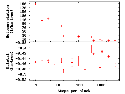
The greatest number of steps per block produces the smallest autocorrelation time. The larger number of blocks over which to average at small step-per-block number masks the corresponding increase in error bar with increasing autocorrelation.
Press q [Enter] to quit gnuplot.
Balancing autocorrelation and acceptance ratio
Adjusting the time step value also affects the ratio of accepted steps to
proposed steps. Stepping nearby in configuration space implies that the
probability distribution is similar and thus more likely to result in an
accepted move. Keeping the acceptance ratio high means the algorithm is
efficiently exploring configuration space and not sticking at particular
configurations. Return to the autocorrelation directory. Refresh your
memory on the time steps in this set of simulations by grep timestep
H.xml. Then, type qmca -q ar *scalar.dat to see the acceptance ratio
as it varies with decreasing time step:
H  series 0  AcceptRatio = 0.047646 +/- 0.000206
H  series 1  AcceptRatio = 0.125361 +/- 0.000308
H  series 2  AcceptRatio = 0.328590 +/- 0.000340
H  series 3  AcceptRatio = 0.535708 +/- 0.000313
H  series 4  AcceptRatio = 0.732537 +/- 0.000234
H  series 5  AcceptRatio = 0.903498 +/- 0.000156
H  series 6  AcceptRatio = 0.961506 +/- 0.000083
H  series 7  AcceptRatio = 0.985499 +/- 0.000051
H  series 8  AcceptRatio = 0.996251 +/- 0.000025
H  series 9  AcceptRatio = 0.998638 +/- 0.000014
H  series 10  AcceptRatio = 0.999515 +/- 0.000009
H  series 11  AcceptRatio = 0.999884 +/- 0.000004
H  series 12  AcceptRatio = 0.999958 +/- 0.000003
H  series 13  AcceptRatio = 0.999986 +/- 0.000002
H  series 14  AcceptRatio = 0.999995 +/- 0.000001
H  series 15  AcceptRatio = 0.999999 +/- 0.000000
By series 8 (time step = 0.02), the acceptance ratio is in excess of 99%.
Considering the increase in autocorrelation and subsequent increase in error bar as time step decreases, it is important to choose a time step that trades off appropriately between acceptance ratio and autocorrelation. In this example, a time step of 0.02 occupies a spot where the acceptance ratio is high (99.6%) and autocorrelation is not appreciably larger than the minimum value (1.4 vs. 1.0).
Considering variance
Besides autocorrelation, the dominant contributor to the error bar is
the variance in the local energy. The variance measures the
fluctuations around the average local energy, and, as the fluctuations
go to zero, the wavefunction reaches an exact eigenstate of the
Hamiltonian. qmca calculates this from the local energy and local energy
squared columns of the scalar.dat.
Type qmca -q v H.s009.scalar.dat to calculate the variance on the
run with time step balancing autocorrelation and acceptance ratio:
H series 9 Variance = 0.513570 +/- 0.010589
Just as the total energy does not tell us much by itself, neither does
the variance. However, comparing the ratio of the variance with the
energy indicates how the magnitude of the fluctuations compares with the
energy itself. Type qmca -q ev H.s009.scalar.dat to calculate the
energy and variance on the run side by side with the ratio:
                    LocalEnergy               Variance        ratio
H  series 0  -0.454460 +/- 0.000568   0.529496 +/- 0.018445   1.1651
The very high ration of 1.1651 indicates the square of the fluctuations is on average larger than the value itself. In the next section, we will approach ways to improve the variance that subsequent labs will build on.
Reducing statistical error bars
Increasing MC sampling
Increasing the number of MC samples in a dataset reduces the error bar as the inverse of the square root of the number of samples. There are two ways to increase the number of MC samples in a simulation: (1) running more samples in parallel and (2) increasing the number of blocks (with fixed number of steps per block, this increases the total number of MC steps).
To see the effect of running more samples in parallel, change to the
directory nodes. The series here increases the number of nodes by
factors of four from 32 to 128 to 512. Type qmca -q ev *scalar.dat
and note the change in the error bar on the local energy as the number
of nodes. Visualize this with gnuplot H.plt:
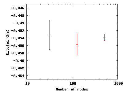
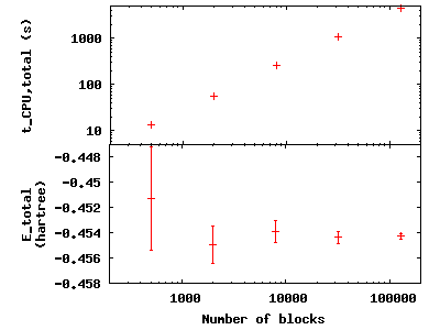
Increasing the number of blocks, unlike running in parallel, increases the total CPU time of the simulation.
Press q [Enter] to quit gnuplot.
To see the effect of increasing the block number, change to the
directory blocks. To see how we will vary the number of blocks, type
grep -A1 blocks H.xml. The number of steps remains fixed, thus
increasing the total number of samples. Visualize the tradeoff by
inputting gnuplot H.plt:
Press q [Enter] to quit gnuplot.
Improving the basis sets
In all of the previous examples, we are using the sum of two Gaussian functions (STO-2G) to approximate what should be a simple decaying exponential for the wavefunction of the ground state of the hydrogen atom. The sum of multiple copies of a function varying each copy’s width and amplitude with coefficients is called a basis set. As we add Gaussians to the basis set, the approximation improves, the variance goes toward zero, and the energy goes to -0.5 Ha. In nearly every other case, the exact function is unknown, and we add basis functions until the total energy does not change within some threshold.
Change to the directory basis and look at the total energy and
variance as we change the wavefunction by typing qmca -q ev H_:
                          LocalEnergy               Variance        ratio
H_STO-2G  series 0  -0.454460 +/- 0.000568   0.529496 +/- 0.018445   1.1651
H_STO-3G  series 0  -0.465386 +/- 0.000502   0.410491 +/- 0.010051   0.8820
H_STO-6G  series 0  -0.471332 +/- 0.000491   0.213919 +/- 0.012954   0.4539
H__exact  series 0  -0.500000 +/- 0.000000   0.000000 +/- 0.000000   -0.0000
qmca also puts out the ratio of the variance to the local energy in a column to the right of the variance error bar. A typical high-quality value for this ratio is lower than 0.1 or so—none of these few-Gaussian wavefunctions satisfy that rule of thumb.
Use qmca to plot the trace of the local energy, kinetic energy, and potential energy of H__exact. The total energy is constantly -0.5 Ha even though the kinetic and potential energies fluctuate from configuration to configuration.
Adding a Jastrow factor
Another route to reducing the variance is the introduction of a Jastrow factor to account for electron-electron correlation (not the statistical autocorrelation of MC steps but the physical avoidance that electrons have of one another). To do this, we will switch to the hydrogen dimer with the exact ground state wavefunction of the atom (STO basis)—this will not be exact for the dimer. The ground state energy of the hydrogen dimer is -1.174 Ha.
Change directories to dimer and put in qmca -q ev *scalar.dat to
see the result of adding a simple, one-parameter Jastrow to the STO
basis for the hydrogen dimer at experimental bond length:
                                LocalEnergy               Variance
H2_STO___no_jastrow  series 0  -0.876548 +/- 0.005313   0.473526 +/- 0.014910
H2_STO_with_jastrow  series 0  -0.912763 +/- 0.004470   0.279651 +/- 0.016405
The energy reduces by 0.044 +/- 0.006 HA and the variance by 0.19 +/- 0.02. This is still 20% above the ground state energy, and subsequent labs will cover how to improve on this with improved forms of the wavefunction that capture more of the physics.
Scaling to larger numbers of electrons
Calculating the efficiency
The inverse of the product of CPU time and the variance measures the
efficiency of an MC calculation. Use qmca to calculate efficiency by
typing qmca -q eff *scalar.dat to see the efficiency of these two
H \(_2\) calculations:
H2_STO___no_jastrow  series 0  Efficiency = 16698.725453 +/- 0.000000
H2_STO_with_jastrow  series 0  Efficiency = 52912.365609 +/- 0.000000
The Jastrow factor increased the efficiency in these calculations by a factor of three, largely through the reduction in variance (check the average block CPU time to verify this claim).
Scaling up
To see how MC scales with increasing particle number, change directories
to size. Here are the data from runs of increasing numbers of
electrons for H, H\(_2\), C, CH\(_4\), C\(_2\),
C\(_2\)H\(_4\), (CH\(_4\))\(_2\), and
(C\(_2\)H\(_4\))\(_2\) using the STO-6G basis set
for the orbitals of the Slater determinant. The file names begin with
the number of electrons simulated for those data.
Use qmca -q bc *scalar.dat to see that the CPU time per block
increases with the number of electrons in the simulation; then plot the
total CPU time of the simulation by gnuplot Nelectron_tCPU.plt:

The green pluses represent the CPU time per block at each electron number. The red line is a quadratic fit to those data. For a fixed basis set size, we expect the time to scale quadratically up to 1,000s of electrons, at which point a cubic scaling term may become dominant. Knowing the scaling allows you to roughly project the calculation time for a larger number of electrons.
Press q [Enter] to quit gnuplot.
This is not the whole story, however. The variance of the energy also
increases with a fixed basis set as the number of particles increases at
a faster rate than the energy decreases. To see this, type
qmca -q ev *scalar.dat:
            LocalEnergy               Variance
01________H  series 0  -0.471352 +/- 0.000493      0.213020 +/- 0.012950
02_______H2  series 0  -0.898875 +/- 0.000998      0.545717 +/- 0.009980
06________C  series 0  -37.608586 +/- 0.020453   184.322000 +/- 45.481193
10______CH4  series 0  -38.821513 +/- 0.022740   169.797871 +/- 24.765674
12_______C2  series 0  -72.302390 +/- 0.037691   491.416711 +/- 106.090103
16_____C2H4  series 0  -75.488701 +/- 0.042919   404.218115 +/- 60.196642
18___CH4CH4  series 0  -58.459857 +/- 0.039309   498.579645 +/- 92.480126
32_C2H4C2H4  series 0  -91.567283 +/- 0.048392   632.114026 +/- 69.637760
The increase in variance is not uniform, but the general trend is upward with a fixed wavefunction form and basis set. Subsequent labs will address how to improve the wavefunction to keep the variance manageable.