Lab 2: QMC Basics
Topics covered in this lab
This lab focuses on the basics of performing quality QMC calculations. As an example, participants test an oxygen pseudopotential within DMC by calculating atomic and dimer properties, a common step prior to production runs. Topics covered include:
Converting pseudopotentials into QMCPACK’s FSATOM format
Generating orbitals with QE
Converting orbitals into QMCPACK’s ESHDF format with pw2qmcpack
Optimizing Jastrow factors with QMCPACK
Removing DMC time step errors via extrapolation
Automating QMC workflows with Nexus
Testing pseudopotentials for accuracy
Lab outline
Download and conversion of oxygen atom pseudopotential
DMC time step study of the neutral oxygen atom
DFT orbital generation with QE
Orbital conversion with
Optimization of Jastrow correlation factor with QMCPACK
DMC run with multiple time steps
DMC time step study of the first ionization potential of oxygen
Repetition of a-d above for ionized oxygen atom
Automated DMC calculations of the oxygen dimer binding curve
Lab directories and files
%
labs/lab2_qmc_basics/
│
├── oxygen_atom           - oxygen atom calculations
│   ├── O.q0.dft.in          - Quantum ESPRESSO input for DFT run
│   ├── O.q0.p2q.in          - pw2qmcpack.x input for orbital conversion run
│   ├── O.q0.opt.in.xml      - QMCPACK input for Jastrow optimization run
│   ├── O.q0.dmc.in.xml      - QMCPACK input file for neutral O DMC
│   ├── ip_conv.py           - tool to fit oxygen IP vs timestep
│   └── reference            - directory w/ completed runs
│
├── oxygen_dimer          - oxygen dimer calculations
│   ├── dimer_fit.py         - tool to fit dimer binding curve
│   ├── O_dimer.py           - automation script for dimer calculations
│   ├── pseudopotentials     - directory for pseudopotentials
│   └── reference            - directory w/ completed runs
│
└── your_system           - performing calculations for an arbitrary system (yours)
    ├── example.py           - example nexus file for periodic diamond
    ├── pseudopotentials     - directory containing C pseudopotentials
    └── reference            - directory w/ completed runs
Obtaining and converting a pseudopotential for oxygen
First enter the oxygen_atom directory:
cd labs/lab2_qmc_basics/oxygen_atom/
Throughout the rest of the lab, locations are specified with respect to labs/lab2_qmc_basics (e.g., oxygen_atom).
We use a potential from the Burkatzki-Filippi-Dolg pseudopotential database.
Although the full database is available in QMCPACK distribution (trunk/pseudopotentials/BFD/),
we use a BFD pseudopotential to illustrate the process of converting and testing an
external potential for use with QMCPACK. To obtain the pseudopotential, go to
http://www.burkatzki.com/pseudos/index.2.html
and click on the “Select Pseudopotential” button. Next click on oxygen in the
periodic table. Click on the empty circle next to “V5Z” (a large Gaussian
basis set) and click on “Next.” Select the Gamess format and click on
“Retrive Potential.” Helpful information about the pseudopotential will be
displayed. The desired portion is at the bottom (the last 7 lines). Copy
this text into the editor of your choice (e.g., emacs or vi)
and save it as O.BFD.gamess
(be sure to include a new line at the end of the file). To transform the
pseudopotential into the FSATOM XML format used by QMCPACK, use the ppconvert
tool:
ppconvert --gamess_pot O.BFD.gamess --s_ref "1s(2)2p(4)" \
 --p_ref "1s(2)2p(4)" --d_ref "1s(2)2p(4)" --xml O.BFD.xml
Observe the notation used to describe the reference valence configuration for this helium-core PP: 1s(2)2p(4). The ppconvert tool uses the following convention for the valence states: the first $s$ state is labeled 1s (1s, 2s, 3s, \(\ldots\)), the first \(p\) state is labeled 2p (2p, 3p, \(\ldots\)), and the first \(d\) state is labeled 3d (3d, 4d, \(\ldots\)). Copy the resulting xml file into the oxygen_atom directory.
Note: The command to convert the PP into QE’s UPF format is similar (both formats are required):
ppconvert --gamess_pot O.BFD.gamess --s_ref "1s(2)2p(4)" \
 --p_ref "1s(2)2p(4)" --d_ref "1s(2)2p(4)" --log_grid --upf O.BFD.upf
For reference, the text of O.BFD.gamess should be:
O-QMC GEN 2 1
3
6.00000000 1 9.29793903
55.78763416 3 8.86492204
-38.81978498 2 8.62925665
1
38.41914135 2 8.71924452
The full QMCPACK pseudopotential is also included in oxygen_atom/reference/O.BFD.*.
DFT with QE to obtain the orbital part of the wavefunction
With the pseudopotential in hand, the next step toward a QMC calculation is to obtain the
Fermionic part of the wavefunction, in this case a single Slater determinant constructed
from DFT-LDA orbitals for a neutral oxygen atom. If you had trouble with the pseudopotential conversion
step, preconverted pseudopotential files are located in the oxygen_atom/reference directory.
QE input for the DFT-LDA ground state of the neutral oxygen atom can be found in O.q0.dft.in
and also in Listing 58. Setting wf_collect=.true. instructs QE to write the
orbitals to disk at the end of the run. Option wf_collect=.true. could be a potential problem
in large simulations; therefore, we recommend avoiding it and using the converter pw2qmcpack in parallel
(see details in pw2qmcpack.x).
Note that the plane-wave energy cutoff has been set to a reasonable value of 300 Ry here (ecutwfc=300).
This value depends on the pseudopotentials used, and, in general,
should be selected by running DFT \(\rightarrow\) (orbital conversion) \(\rightarrow\) VMC with
increasing energy cutoffs until the lowest VMC total energy and variance is reached.
&CONTROL
   calculation       = 'scf'
   restart_mode      = 'from_scratch'
   prefix            = 'O.q0'
   outdir            = './'
   pseudo_dir        = './'
   disk_io           = 'low'
   wf_collect        = .true.
/

&SYSTEM
   celldm(1)         = 1.0
   ibrav             = 0
   nat               = 1
   ntyp              = 1
   nspin             = 2
   tot_charge        = 0
   tot_magnetization = 2
   input_dft         = 'lda'
   ecutwfc           = 300
   ecutrho           = 1200
   nosym             = .true.
   occupations       = 'smearing'
   smearing          = 'fermi-dirac'
   degauss           = 0.0001
/

&ELECTRONS
   diagonalization   = 'david'
   mixing_mode       = 'plain'
   mixing_beta       = 0.7
   conv_thr          = 1e-08
   electron_maxstep  = 1000
/


ATOMIC_SPECIES
   O  15.999 O.BFD.upf

ATOMIC_POSITIONS alat
   O     9.44863067       9.44863161       9.44863255

K_POINTS automatic
   1 1 1  0 0 0

CELL_PARAMETERS cubic
        18.89726133       0.00000000       0.00000000
         0.00000000      18.89726133       0.00000000
         0.00000000       0.00000000      18.89726133
Run QE by typing
mpirun -np 4 pw.x -input O.q0.dft.in >&O.q0.dft.out&
The DFT run should take a few minutes to complete. If desired, you can track the progress of the DFT run by typing “tail -f O.q0.dft.out.” Once finished, you should check the LDA total energy in O.q0.dft.out by typing “grep '! ' O.q0.dft.out.” The result should be close to
! total energy = -31.57553905 Ry
The orbitals have been written in a format native to QE in the O.q0.save directory. We will convert them into the ESHDF format expected by QMCPACK by using the pw2qmcpack.x tool. The input for pw2qmcpack.x can be found in the file O.q0.p2q.in and also in Listing 59.
&inputpp
  prefix     = 'O.q0'
  outdir     = './'
  write_psir = .false.
/
Perform the orbital conversion now by typing the following:
mpirun -np 1 pw2qmcpack.x<O.q0.p2q.in>&O.q0.p2q.out&
Upon completion of the run, a new file should be present containing the orbitals for QMCPACK: O.q0.pwscf.h5. Template XML files for particle (O.q0.ptcl.xml) and wavefunction (O.q0.wfs.xml) inputs to QMCPACK should also be present.
DMC timestep extrapolation I: neutral oxygen atom
The DMC algorithm contains two biases in addition to the fixed node and pseudopotential approximations that are important to control: time step and population control bias. In this section we focus on estimating and removing time step bias from DMC calculations. The essential fact to remember is that the bias vanishes as the time step goes to zero, while the needed computer time increases inversely with the time step.
In the same directory you used to perform wavefunction optimization (oxygen_atom) you will find a sample DMC input file for the neutral oxygen atom named O.q0.dmc.in.xml. Open this file in a text editor and note the differences from the optimization case. Wavefunction information is no longer included from pw2qmcpack but instead should come from the optimization run:
<!-- OPT_XML is from optimization, e.g. O.q0.opt.s008.opt.xml -->
<include href="OPT_XML"/>
Replace “OPT_XML” with the opt.xml file corresponding to the best Jastrow parameters you found in the last section (this is a file name similar to O.q0.opt.s008.opt.xml).
The QMC calculation section at the bottom is also different. The linear optimization blocks have been replaced with XML describing a VMC run followed by DMC. Descriptions of the input keywords follow.
- timestep
Time step of the VMC/DMC random walk. In VMC choose a time step corresponding to an acceptance ratio of about 50%. In DMC the acceptance ratio is often above 99%.
- warmupSteps
Number of MC steps discarded as a warmup or equilibration period of the random walk.
- steps
Number of MC steps per block. Physical quantities, such as the total energy, are averaged over walkers and steps.
- blocks
Number of blocks. This is also the number of average energy values written to output files. The number should be greater than 200 for meaningful statistical analysis of output data (e.g., via
qmca). The total number of MC steps each walker takes isblocks\(\times\)steps.- samples
VMC only. This is the number of walkers used in subsequent DMC runs. Each DMC walker is initialized with electron positions sampled from the VMC random walk.
- nonlocalmoves
DMC only. If yes/no, use the locality approximation/T-moves for nonlocal pseudopotentials. T-moves generally improve the stability of the algorithm and restore the variational principle for small systems (T-moves version 1).
The purpose of the VMC run is to provide initial electron positions for each DMC walker. Setting \(\texttt{walkers}=1\) in the VMC block ensures there will be only one VMC walker per execution thread. There will be a total of 4 VMC walkers in this case (see O.q0.dmc.qsub.in). We want the electron positions used to initialize the DMC walkers to be decorrelated from one another. A VMC walker will often decorrelate from its current position after propagating for a few Ha \(^{-1}\) in imaginary time (in general, this is system dependent). This leads to a rough rule of thumb for choosing blocks and steps for the VMC run (\(\texttt{vwalkers}=4\) here):
Fill in the VMC XML block with appropriate values for these parameters. There should be more than one DMC walker per thread and enough walkers in total to avoid population control bias. The general rule of thumb is to have more than \(\sim 2,000\) walkers, although the dependence of the total energy on population size should be explicitly checked from time to time.
To study time step bias, we will perform a sequence of DMC runs over a range of time steps (\(0.1\) Ha\(^{-1}\) is too large, and time steps below \(0.002\) Ha\(^{-1}\) are probably too small). A common approach is to select a fairly large time step to begin with and then decrease the time step by a factor of two in each subsequent DMC run. The total amount of imaginary time the walker population propagates should be the same for each run. A simple way to accomplish this is to choose input parameters in the following way
Each DMC run will require about twice as much computer time as the one preceding it. Note that the number of blocks is kept fixed for uniform statistical analysis. \(\texttt{blocks}\times\texttt{steps}\times\texttt{timestep}\sim 60~\mathrm{Ha}^{-1}\) is sufficient for this system.
Choose an initial DMC time step and create a sequence of \(N\) time steps according to (75). Make \(N\) copies of the DMC XML block in the input file.
<qmc method="dmc" move="pbyp">
   <parameter name="warmupSteps"         >    DWARMUP         </parameter>
   <parameter name="blocks"              >    DBLOCKS         </parameter>
   <parameter name="steps"               >    DSTEPS          </parameter>
   <parameter name="timestep"            >    DTIMESTEP       </parameter>
   <parameter name="nonlocalmoves"       >    yes             </parameter>
</qmc>
Fill in DWARMUP, DBLOCKS, DSTEPS, and DTIMESTEP for each DMC run according to (75). Start the DMC time step extrapolation run by typing:
mpirun -np 4 qmcpack O.q0.dmc.in.xml >&O.q0.dmc.out&
The run should take only a few minutes to complete.
QMCPACK will create files prefixed with O.q0.dmc. The log file is O.q0.dmc.out. As before, block-averaged data is written to scalar.dat files. In addition, DMC runs produce dmc.dat files, which contain energy data averaged only over the walker population (one line per DMC step). The dmc.dat files also provide a record of the walker population at each step.
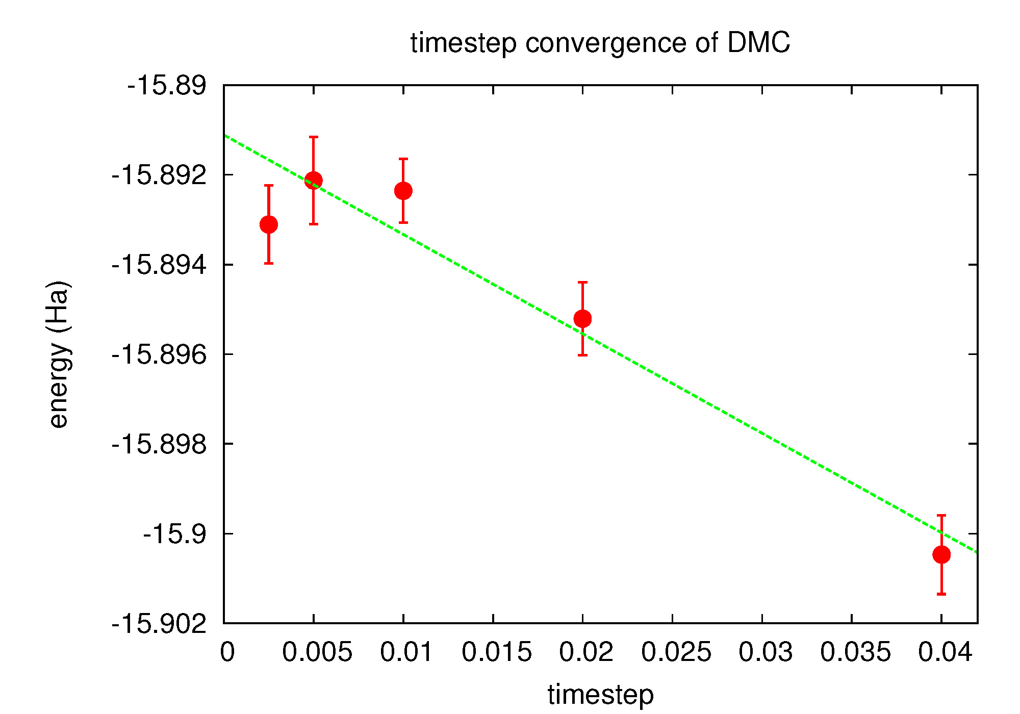
Fig. 16 Linear fit to DMC timestep data from PlotTstepConv.pl.
Use the PlotTstepConv.pl to obtain a linear fit to the time step data (type “PlotTstepConv.pl O.q0.dmc.in.xml 40”). You should see a plot similar to Fig. 16. The tail end of the text output displays the parameters for the linear fit. The “a” parameter is the total energy extrapolated to zero time step in Hartree units.
...
Final set of parameters            Asymptotic Standard Error
=======================            ==========================

a               = -15.8925         +/- 0.0007442    (0.004683%)
b               = -0.0457479       +/- 0.0422       (92.24%)
...
Questions and Exercises
What is the \(\tau\rightarrow 0\) extrapolated value for the total energy?
What is the maximum time step you should use if you want to calculate the total energy to an accuracy of \(0.05\) eV? For convenience, \(1~\textrm{Ha}=27.2113846~\textrm{eV}\).
What is the acceptance ratio for this (bias \(<0.05\) eV) run? Does it follow the rule of thumb for sensible DMC (acceptance ratio \(>99\)%) ?
Check the fluctuations in the walker population (
qmca -t -q nw O.q0.dmc*dmc.dat –noac). Does the population seem to be stable?(Optional) Study population control bias for the oxygen atom. Select a few population sizes. Copy
O.q0.dmc.in.xmlto a new file and remove all but one DMC run (select a single time step). Make one copy of the new file for each population, set “textttsamples,” and choose a uniqueidin<project/>. Useqmcato study the dependence of the DMC total energy on the walker population. How large is the bias compared with time step error? What bias is incurred by following the “rule of thumb” of a couple thousand walkers? Will population control bias generally be an issue for production runs on modern parallel machines?
DMC time step extrapolation II: oxygen atom ionization potential
In this section, we will repeat the calculations of the previous two sections (optimization, time step extrapolation) for the \(+1\) charge state of the oxygen atom. Comparing the resulting first ionization potential (IP) with experimental data will complete our first test of the BFD oxygen pseudopotential. In actual practice, higher IPs could also be tested before performing production runs.
Obtaining the time step extrapolated DMC total energy for ionized oxygen should take much less (human) time than for the neutral case. For convenience, the necessary steps are summarized as follows.
Obtain DFT orbitals with QE.
Copy the DFT input (
O.q0.dft.in) toO.q1.dft.inEdit
O.q1.dft.into match the +1 charge state of the oxygen atom.... prefix = 'O.q1' ... tot_charge = 1 tot_magnetization = 3 ...
Perform the DFT run:
mpirun -np 4 pw.x -input O.q1.dft.in >&O.q1.dft.out&
Convert the orbitals to ESHDF format.
Copy the pw2qmcpack input (
O.q0.p2q.in) toO.q1.p2q.inEdit
O.q1.p2q.into match the file prefix used in DFT.... prefix = 'O.q1' ...
Perform the orbital conversion run:
mpirun -np 1 pw2qmcpack.x<O.q1.p2q.in>&O.q1.p2q.out&
Optimize the Jastrow factor with QMCPACK.
Copy the optimization input (
O.q0.opt.in.xml) toO.q1.opt.in.xmlEdit
O.q1.opt.in.xmlto match the file prefix used in DFT.... <project id="O.q1.opt" series="0"> ... <include href="O.q1.ptcl.xml"/> ... <include href="O.q1.wfs.xml"/> ...
Edit the particle XML file (
O.q1.ptcl.xml) to have open boundary conditions.<parameter name="bconds"> n n n </parameter>
Add cutoffs to the Jastrow factors in the wavefunction XML file (
O.q1.wfs.xml)... <correlation speciesA="u" speciesB="u" size="8" rcut="10.0"> ... <correlation speciesA="u" speciesB="d" size="8" rcut="10.0"> ... <correlation elementType="O" size="8" rcut="5.0"> ...
Perform the Jastrow optimization run:
mpirun -np 4 qmcpack O.q1.opt.in.xml >&O.q1.opt.out&Identify the optimal set of parameters with
qmca([your opt.xml]).
DMC time step study with QMCPACK
Copy the DMC input (
O.q0.dmc.in.xml) toO.q1.dmc.in.xmlEdit
O.q1.dmc.in.xmlto use the DFT prefix and the optimal Jastrow.... <project id="O.q1.dmc" series="0"> ... <include href="O.q1.ptcl.xml"/> ... <include href="[your opt.xml]"/> ...
Perform the DMC run:
mpirun -np 4 qmcpack O.q1.dmc.in.xml >&O.q1.dmc.out&Obtain the DMC total energy extrapolated to zero time step with
PlotTstepConv.pl.
The aforementioned process, which excludes additional steps for orbital generation and conversion, can become tedious to perform by hand in production settings where many calculations are often required. For this reason, automation tools are introduced for calculations involving the oxygen dimer in Automated binding curve of the oxygen dimer of the lab.
Questions and Exercises
What is the \(\tau\rightarrow 0\) extrapolated DMC value for the first ionization potential of oxygen?
How does the extrapolated value compare with the experimental IP? Go to http://physics.nist.gov/PhysRefData/ASD/ionEnergy.html and enter “
O I” in the box labeled “Spectra” and click on the “Retrieve Data” button.What can we conclude about the accuracy of the pseudopotential? What factors complicate this assessment?
Explore the sensitivity of the IP to the choice of time step. Type
./ip_conv.pyto view three time step extrapolation plots: two for the \(q=0,\) one for total energies, and one for the IP. Is the IP more, less, or similarly sensitive to time step than the total energy?What is the maximum time step you should use if you want to calculate the ionization potential to an accuracy of \(0.05\) eV? What factor of CPU time is saved by assessing time step convergence on the IP (a total energy difference) vs. a single total energy?
Are the acceptance ratio and population fluctuations reasonable for the \(q=1\) calculations?
DMC workflow automation with Nexus
Production QMC projects are often composed of many similar workflows. The simplest of these is a single DMC calculation involving four different compute jobs:
Orbital generation via QE or GAMESS.
Conversion of orbital data via
pw2qmcpack.xorconvert4qmc.Optimization of Jastrow factors via QMCPACK.
DMC calculation via QMCPACK.
Simulation workflows quickly become more complex with increasing costs in terms of human time for the researcher. Automation tools can decrease both human time and error if used well.
The set of automation tools we will be using is known as Nexus [Kro16], which is distributed with QMCPACK. Nexus is capable of generating input files, submitting and monitoring compute jobs, passing data between simulations (relaxed structures, orbital files, optimized Jastrow parameters, etc.), and data analysis. The user interface to Nexus is through a set of functions defined in the Python programming language. User scripts that execute simple workflows resemble input files and do not require programming experience. More complex workflows require only basic programming constructs (e.g. for loops and if statements). Nexus input files/scripts should be easier to navigate than QMCPACK input files and more efficient than submitting all the jobs by hand.
Nexus is driven by simple user-defined scripts that resemble keyword-driven input files. An example Nexus input file that performs a single VMC calculation (with pregenerated orbitals) follows. Take a moment to read it over and especially note the comments (prefixed with “\#”) explaining most of the contents. If the input syntax is unclear you may want to consult portions of Appendix A: Basic Python constructs, which gives a condensed summary of Python constructs. An additional example and details about the inner workings of Nexus can be found in the reference publication [Kro16].
#! /usr/bin/env python3

# import Nexus functions
from nexus import settings,job,get_machine,run_project
from nexus import generate_physical_system
from nexus import generate_qmcpack,vmc

settings(                             # Nexus settings
    pseudo_dir    = './pseudopotentials', # location of PP files
    runs          = '',                   # root directory for simulations
    results       = '',                   # root directory for simulation results
    status_only   = 0,                    # show simulation status, then exit
    generate_only = 0,                    # generate input files, then exit
    sleep         = 3,                    # seconds between checks on sim. progress
    machine       = 'ws4',                # workstation with 4 cores
    )

qmcjob = job(                         # specify job parameters
    cores   = 4,                          # use 4 MPI tasks
    threads = 1,                          # 1 OpenMP thread per node
    app     = 'qmcpack'                   # use QMCPACK executable (assumed in PATH)
    )

qmc_calcs = [                         # list QMC calculation methods
    vmc(                                  #   VMC
        walkers     =   1,                #     1 walker
        warmupsteps =  50,                #    50 MC steps for warmup
        blocks      = 200,                #   200 blocks
        steps       =  10,                #    10 steps per block
        timestep    =  .4                 #   0.4 1/Ha timestep
        )]

dimer = generate_physical_system(     # make a dimer system
    type       = 'dimer',                 # system type is dimer
    dimer      = ('O','O'),               # dimer is two oxygen atoms
    separation = 1.2074,                  # separated by 1.2074 Angstrom
    Lbox       = 15.0,                    # simulation box is 15 Angstrom
    units      = 'A',                     # Angstrom is dist. unit
    net_spin   = 2,                       # nup-ndown is 2
    O          = 6                        # pseudo-oxygen has 6 valence el.
    )

qmc = generate_qmcpack(                # make a qmcpack simulation
    identifier   = 'example',             # prefix files with 'example'
    path         = 'scale_1.0',           # run in ./scale_1.0 directory
    system       = dimer,                 # run the dimer system
    job          = qmcjob,                # set job parameters
    input_type   = 'basic',               # basic qmcpack inputs given below
    pseudos      = ['O.BFD.xml'],         # list of PP's to use
    orbitals_h5  = 'O2.pwscf.h5',         # file with orbitals from DFT
    bconds       = 'nnn',                 # open boundary conditions
    jastrows     = [],                    # no jastrow factors
    calculations = qmc_calcs              # QMC calculations to perform
    )

run_project(qmc)                       # write input file and submit job
Automated binding curve of the oxygen dimer
In this section we will use Nexus to calculate the DMC total energy of the oxygen dimer over a series of bond lengths. The equilibrium bond length and binding energy of the dimer will be determined by performing a polynomial fit to the data (Morse potential fits should be preferred in production tests). Comparing these values with corresponding experimental data provides a second test of the BFD pseudopotential for oxygen.
Enter the oxygen_dimer directory. Copy your BFD pseudopotential from the atom runs into oxygen_dimer/pseudopotentials (be sure to move both files: .upf and .xml). Open O_dimer.py with a text editor. The overall format is similar to the example file shown in the last section. The main difference is that a full workflow of runs (DFT orbital generation, orbital conversion, optimization and DMC) are being performed rather than a single VMC run.
As in the example in the last section, the oxygen dimer is generated with the generate_physical_
system function:
dimer = generate_physical_system(
    type       = 'dimer',
    dimer      = ('O','O'),
    separation = 1.2074*scale,
    Lbox       = 10.0,
    units      = 'A',
    net_spin   = 2,
    O          = 6
    )
Similar syntax can be used to generate crystal structures or to specify systems with arbitrary atomic configurations and simulation cells. Notice that a “scale” variable has been introduced to stretch or compress the dimer.
Next, objects representing a QE (PWSCF) run and subsequent orbital conversion step are constructed with respective generate_* functions:
dft = generate_pwscf(
    identifier   = 'dft',
    ...
    input_dft    = 'lda',
    ...
    )
sims.append(dft)

# describe orbital conversion run
p2q = generate_pw2qmcpack(
    identifier   = 'p2q',
    ...
    dependencies = (dft,'orbitals'),
    )
sims.append(p2q)
Note the dependencies keyword. This keyword is used to construct workflows out of otherwise separate runs. In this case, the dependency indicates that the orbital conversion run must wait for the DFT to finish before starting.
Objects representing QMCPACK simulations are then constructed with the generate_qmcpack function:
opt = generate_qmcpack(
    identifier   = 'opt',
    ...
    jastrows     = [('J1','bspline',8,5.0),
                    ('J2','bspline',8,10.0)],
    calculations = [
        loop(max=12,
             qmc=linear(
                energy               = 0.0,
                unreweightedvariance = 1.0,
                reweightedvariance   = 0.0,
                timestep             = 0.3,
                samples              = 61440,
                warmupsteps          = 50,
                blocks               = 200,
                substeps             = 1,
                nonlocalpp           = True,
                usebuffer            = True,
                walkers              = 1,
                minwalkers           = 0.5,
                maxweight            = 1e9,
                usedrift             = False,
                minmethod            = 'quartic',
                beta                 = 0.025,
                exp0                 = -16,
                bigchange            = 15.0,
                alloweddifference    = 1e-4,
                stepsize             = 0.2,
                stabilizerscale      = 1.0,
                nstabilizers         = 3,
                )
             )
        ],
    dependencies = (p2q,'orbitals'),
    )
sims.append(opt)

qmc = generate_qmcpack(
    identifier   = 'qmc',
    ...
    jastrows     = [],
    calculations = [
        vmc(
            walkers     =   1,
            warmupsteps =  30,
            blocks      =  20,
            steps       =  10,
            substeps    =   2,
            timestep    =  .4,
            samples     = 2048
            ),
        dmc(
            warmupsteps   = 100,
            blocks        = 400,
            steps         =  32,
            timestep      = 0.01,
            nonlocalmoves = True,
            )
        ],
    dependencies = [(p2q,'orbitals'),(opt,'jastrow')],
    )
sims.append(qmc)
Shared details such as the run directory, job, pseudopotentials, and orbital file have been omitted (...). The “opt” run will optimize a 1-body B-spline Jastrow with 8 knots having a cutoff of 5.0 Bohr and a B-spline Jastrow (for up-up and up-down correlations) with 8 knots and cutoffs of 10.0 Bohr. The Jastrow list for the DMC run is empty, and the previous use of dependencies indicates that the DMC run depends on the optimization run for the Jastrow factor. Nexus will submit the “opt” run first, and upon completion it will scan the output, select the optimal set of parameters, pass the Jastrow information to the “qmc” run, and then submit the DMC job. Independent job workflows are submitted in parallel when permitted. No input files are written or job submissions made until the “run_project” function is reached:
run_project(sims)
All of the simulation objects have been collected into a list (sims) for submission.
As written, O_dimer.py will perform calculations only at the equilibrium separation distance of 1.2074 {AA} since the list of scaling factors (representing stretching or compressing the dimer) contains only one value (scales = [1.00]). Modify the file now to perform DMC calculations across a range of separation distances with each DMC run using the Jastrow factor optimized at the equilibrium separation distance. Specifically, you will want to change the list of scaling factors to include both compression (scale<1.0) and stretch (scale>1.0):
scales = [1.00,0.90,0.95,1.05,1.10]
Note that “1.00” is left in front because we are going to optimize the Jastrow factor first at the equilibrium separation and reuse this Jastrow factor for all other separation distances. This procedure is used because it can reduce variations in localization errors (due to pseudopotentials in DMC) along the binding curve.
Change the status_only parameter in the “settings” function to 1 and type “./O_dimer.py” at the command line. This will print the status of all simulations:
Project starting
  checking for file collisions
  loading cascade images
    cascade 0 checking in
    cascade 10 checking in
    cascade 4 checking in
    cascade 13 checking in
    cascade 7 checking in
  checking cascade dependencies
    all simulation dependencies satisfied

  cascade status
    setup, sent_files, submitted, finished, got_output, analyzed
    000000  dft     ./scale_1.0
    000000  p2q     ./scale_1.0
    000000  opt     ./scale_1.0
    000000  qmc     ./scale_1.0
    000000  dft     ./scale_0.9
    000000  p2q     ./scale_0.9
    000000  qmc     ./scale_0.9
    000000  dft     ./scale_0.95
    000000  p2q     ./scale_0.95
    000000  qmc     ./scale_0.95
    000000  dft     ./scale_1.05
    000000  p2q     ./scale_1.05
    000000  qmc     ./scale_1.05
    000000  dft     ./scale_1.1
    000000  p2q     ./scale_1.1
    000000  qmc     ./scale_1.1
    setup, sent_files, submitted, finished, got_output, analyzed
In this case, five simulation “cascades” (workflows) have been identified, each one starting and ending with “dft” and “qmc” runs, respectively. The six status flags setup, sent_files, submitted, finished, got_output, analyzed) each shows 0, indicating that no work has been done yet.
Now change “status_only” back to 0, set “generate_only” to 1, and run O_dimer.py again. This will perform a dry run of all simulations. The dry run should finish in about 20 seconds:
Project starting
  checking for file collisions
  loading cascade images
    cascade 0 checking in
    cascade 10 checking in
    cascade 4 checking in
    cascade 13 checking in
    cascade 7 checking in
  checking cascade dependencies
    all simulation dependencies satisfied

  starting runs:
  ~~~~~~~~~~~~~~~~~~~~~~~~~~~~~~
  poll 0  memory 91.03 MB
    Entering ./scale_1.0 0
      writing input files  0 dft
    Entering ./scale_1.0 0
      sending required files  0 dft
      submitting job  0 dft
  ...
  poll 1  memory 91.10 MB
  ...
    Entering ./scale_1.0 0
      Would have executed:
        export OMP_NUM_THREADS=1
        mpirun -np 4 pw.x -input dft.in

  poll 2  memory 91.10 MB
    Entering ./scale_1.0 0
      copying results  0 dft
    Entering ./scale_1.0 0
      analyzing  0 dft
  ...
  poll 3  memory 91.10 MB
    Entering ./scale_1.0 1
      writing input files  1 p2q
    Entering ./scale_1.0 1
      sending required files  1 p2q
      submitting job  1 p2q
  ...
    Entering ./scale_1.0 1
      Would have executed:
        export OMP_NUM_THREADS=1
        mpirun -np 1 pw2qmcpack.x<p2q.in

  poll 4  memory 91.10 MB
    Entering ./scale_1.0 1
      copying results  1 p2q
    Entering ./scale_1.0 1
      analyzing  1 p2q
  ...
  poll 5  memory 91.10 MB
    Entering ./scale_1.0 2
      writing input files  2 opt
    Entering ./scale_1.0 2
      sending required files  2 opt
      submitting job  2 opt
  ...
    Entering ./scale_1.0 2
      Would have executed:
        export OMP_NUM_THREADS=1
        mpirun -np 4 qmcpack opt.in.xml

  poll 6  memory 91.16 MB
    Entering ./scale_1.0 2
      copying results  2 opt
    Entering ./scale_1.0 2
      analyzing  2 opt
  ...
  poll 7  memory 93.00 MB
    Entering ./scale_1.0 3
      writing input files  3 qmc
    Entering ./scale_1.0 3
      sending required files  3 qmc
      submitting job  3 qmc
  ...
    Entering ./scale_1.0 3
      Would have executed:
        export OMP_NUM_THREADS=1
        mpirun -np 4 qmcpack qmc.in.xml
  ...
  poll 17  memory 93.06 MB
Project finished
Nexus polls the simulation status every 3 seconds and sleeps in between.
The “scale_” directories should now contain several files:
scale_1.0
   dft.in
   O.BFD.upf
   O.BFD.xml
   opt.in.xml
   p2q.in
   pwscf_output
   qmc.in.xml
   sim_dft/
       analyzer.p
       input.p
       sim.p
   sim_opt/
       analyzer.p
       input.p
       sim.p
   sim_p2q/
       analyzer.p
       input.p
       sim.p
   sim_qmc/
       analyzer.p
       input.p
       sim.p
Take a minute to inspect the generated input (dft.in, p2q.in, opt.in.xml, qmc.in.xml). The pseudopotential files (O.BFD.upf and O.BFD.xml) have been copied into each local directory. Four additional directories have been created: sim_dft, sim_p2q, sim_opt and sim_qmc. The sim.p files in each directory contain the current status of each simulation. If you run O_dimer.py again, it should not attempt to rerun any of the simulations:
Project starting
  checking for file collisions
  loading cascade images
    cascade 0 checking in
    cascade 10 checking in
    cascade 4 checking in
    cascade 13 checking in
    cascade 7 checking in
  checking cascade dependencies
    all simulation dependencies satisfied

  starting runs:
  ~~~~~~~~~~~~~~~~~~~~~~~~~~~~~~
  poll 0  memory 64.25 MB
Project finished
This way you can continue to add to the O_dimer.py file (e.g., adding more separation distances) without worrying about duplicate job submissions.
Now submit the jobs in the dimer workflow. Reset the state of the simulations by removing the sim.p files (”rm ./scale*/sim*/sim.p”), set “generate_only” to 0, and rerun O_dimer.py. It should take about 20 minutes for all the jobs to complete. You may wish to open another terminal to monitor the progress of the individual jobs while the current terminal runs O_dimer.py in the foreground. You can begin the following first exercise once the optimization job completes.
Questions and Exercises
Evaluate the quality of the optimization at
scale=1.0using theqmcatool. Did the optimization succeed? How does the variance compare with the neutral oxygen atom? Is the wavefunction of similar quality to the atomic case?Evaluate the traces of the local energy and the DMC walker population for each separation distance with the
qmcatool. Are there any anomalies in the runs? Is the acceptance ratio reasonable? Is the wavefunction of similar quality across all separation distances?Use the
dimer_fit.pytool located inoxygen_dimerto fit the oxygen dimer binding curve. To get the binding energy of the dimer, we will need the DMC energy of the atom. Before performing the fit, answer: What DMC time step should be used for the oxygen atom results? The tool accepts three arguments (./dimer_fit.py P N E Eerr),Pis the prefix of the DMC input files (should be “qmc” at this point),Nis the order of the fit (use 2 to start),``E`` andEerrare your DMC total energy and error bar, respectively, for the oxygen atom (in electron volts). A plot of the dimer data will be displayed, and text output will show the DMC equilibrium bond length and binding energy as well as experimental values. How accurately does your fit to the DMC data reproduce the experimental values? What factors affect the accuracy of your results?Refit your data with a fourth-order polynomial. How do your predictions change with a fourth-order fit? Is a fourth-order fit appropriate for the available data?
Add new “
scale” values to the list inO_dimer.pythat interpolate between the original set (e.g., expand to ). Perform the DMC calculations and redo the fits. How accurately does your fit to the DMC data reproduce the experimental values? Should this pseudopotential be used in production calculations?(Optional) Perform optimization runs at the extreme separation distances corresponding to
scale=[0.90,1.10]. Are the individually optimized wavefunctions of significantly better quality than the one imported fromscale=1.00? Why? What form of Jastrow factor might give an even better improvement?
(Optional) Running your system with QMCPACK
This section covers a fairly simple route to get started on QMC calculations of an arbitrary system of interest using the Nexus workflow management system to set up input files and optionally perform the runs. The example provided in this section uses QE (PWSCF) to generate the orbitals forming the Slater determinant part of the trial wavefunction. PWSCF is a natural choice for solid-state systems, and it can be used for surface/slab and molecular systems as well, albeit at the price of describing additional vacuum space with plane waves.
To start out, you will need PPs for each element in your system in both
the UPF (PWSCF) and FSATOM/XML (QMCPACK) formats. A good place to start
is the BFD pseudopotential database
(http://www.burkatzki.com/pseudos/index.2.html), which we have already
used in our study of the oxygen atom. The database does not contain PPs
for the fourth and fifth row transition metals or any of the lanthanides
or actinides. If you need a PP that is not in the BFD database, you may
need to generate and test one manually (e.g., with OPIUM,
http://opium.sourceforge.net/). Otherwise, use ppconvert as outlined in
Obtaining and converting a pseudopotential for oxygen to obtain PPs in the formats used by PWSCF
and QMCPACK. Enter the your_system lab directory and place the converted PPs in your_system/pseudopotentials.
Before performing production calculations (more than just the initial setup in this section), be sure to converge the plane-wave energy cutoff in PWSCF as these PPs can be rather hard, sometimes requiring cutoffs in excess of 300 Ry. Depending on the system under study, the amount of memory required to represent the orbitals (QMCPACK uses 3D B-splines) can become prohibitive, forcing you to search for softer PPs.
Beyond PPs, all that is required to get started are the atomic positions and the dimensions/shape of the simulation cell. The Nexus file example.py illustrates how to set up PWSCF and QMCPACK input files by providing minimal information regarding the physical system (an 8-atom cubic cell of diamond in the example). Most of the contents should be familiar from your experience with the automated calculations of the oxygen dimer binding curve in Automated binding curve of the oxygen dimer (if you have skipped ahead you may want to skim that section for relevant information). The most important change is the expanded description of the physical system:
# details of your physical system (diamond conventional cell below)
my_project_name = 'diamond_vmc'   # directory to perform runs
my_dft_pps      = ['C.BFD.upf']   # pwscf pseudopotentials
my_qmc_pps      = ['C.BFD.xml']   # qmcpack pseudopotentials

#  generate your system
#    units      :  'A'/'B' for Angstrom/Bohr
#    axes       :  simulation cell axes in cartesian coordinates (a1,a2,a3)
#    elem       :  list of atoms in the system
#    pos        :  corresponding atomic positions in cartesian coordinates
#    kgrid      :  Monkhorst-Pack grid
#    kshift     :  Monkhorst-Pack shift (between 0 and 0.5)
#    net_charge :  system charge in units of e
#    net_spin   :  # of up spins - # of down spins
#    C = 4      :  (pseudo) carbon has 4 valence electrons
my_system = generate_physical_system(
    units      = 'A',
    axes       = [[ 3.57000000e+00, 0.00000000e+00, 0.00000000e+00],
                  [ 0.00000000e+00, 3.57000000e+00, 0.00000000e+00],
                  [ 0.00000000e+00, 0.00000000e+00, 3.57000000e+00]],
    elem       = ['C','C','C','C','C','C','C','C'],
    pos        = [[ 0.00000000e+00, 0.00000000e+00, 0.00000000e+00],
                  [ 8.92500000e-01, 8.92500000e-01, 8.92500000e-01],
                  [ 0.00000000e+00, 1.78500000e+00, 1.78500000e+00],
                  [ 8.92500000e-01, 2.67750000e+00, 2.67750000e+00],
                  [ 1.78500000e+00, 0.00000000e+00, 1.78500000e+00],
                  [ 2.67750000e+00, 8.92500000e-01, 2.67750000e+00],
                  [ 1.78500000e+00, 1.78500000e+00, 0.00000000e+00],
                  [ 2.67750000e+00, 2.67750000e+00, 8.92500000e-01]],
    kgrid      = (1,1,1),
    kshift     = (0,0,0),
    net_charge = 0,
    net_spin   = 0,
    C          = 4       # one line like this for each atomic species
    )

my_bconds       = 'ppp'  #  ppp/nnn for periodic/open BC's in QMC
                         #  if nnn, center atoms about (a1+a2+a3)/2
If you have a system you would like to try with QMC, make a copy of example.py and fill in the relevant information about the PPs, simulation cell axes, and atomic species/positions. Otherwise, you can proceed with example.py as it is.
Set “generate_only” to 1 and type “./example.py” or similar to generate the input files. All files will be written to “./diamond_vmc” (”./[my_project_name]” if you have changed “my_project_name” in the file). The input files for PWSCF, pw2qmcpack, and QMCPACK are scf.in, pw2qmcpack.in, and vmc.in.xml, respectively. Take some time to inspect the generated input files. If you have questions about the file contents, or run into issues with the generation process, feel free to consult with a lab instructor.
If desired, you can submit the runs directly with example.py. To do this, first reset the Nexus simulation record by typing “rm ./diamond_vmc/sim*/sim.p” or similar and set “generate_only” back to 0. Next rerun example.py (you may want to redirect the text output).
Alternatively the runs can be submitted by hand:
mpirun -np 4 pw.x<scf.in>&scf.out&

(wait until JOB DONE appears in scf.out)

mpirun -np 1 pw2qmcpack.x<p2q.in>&p2q.out&
Once the conversion process has finished, the orbitals should be located in the file diamond_vmc/pwscf_output/pwscf.pwscf.h5. Open diamond_vmc/vmc.in.xml and replace “MISSING.h5” with “./pwscf_output/pwscf.pwscf.h5”. Next submit the VMC run:
mpirun -np 4 qmcpack vmc.in.xml>&vmc.out&
Note: If your system is large, the preceding process may not complete within the time frame of this lab. Working with a stripped down (but relevant) example is a good idea for exploratory runs.
Once the runs have finished, you may want to begin exploring Jastrow optimization and DMC for your system. Example calculations are provided at the end of example.py in the commented out text.
Appendix A: Basic Python constructs
Basic Python data types (int, float, str, tuple, list, array, dict, obj) and programming constructs (if statements, for loops, functions w/ keyword arguments) are briefly overviewed in the following. All examples can be executed interactively in Python. To do this, type “python” at the command line and paste any of the shaded text below at the >>> prompt. For more information about effective use of Python, consult the detailed online documentation: https://docs.python.org/2/.
Intrinsic types: int, float, str
#this is a comment
i=5                     # integer
f=3.6                   # float
s='quantum/monte/carlo' # string
n=None                  # represents "nothing"

f+=1.4                  # add-assign (-,*,/ also): 5.0
2**3                    # raise to a power: 8
str(i)                  # int to string: '5'
s+'/simulations'        # joining strings: 'quantum/monte/carlo/simulations'
'i={0}'.format(i)       # format string: 'i=5'
Container types: tuple, list, array, dict, obj
from numpy import array  # get array from numpy module
from generic import obj  # get obj from Nexus' generic module

t=('A',42,56,123.0)     # tuple

l=['B',3.14,196]        # list

a=array([1,2,3])        # array

d={'a':5,'b':6}         # dict

o=obj(a=5,b=6)          # obj

                        # printing
print(t)                #  ('A', 42, 56, 123.0)
print(l)                #  ['B', 3.1400000000000001, 196]
print(a)                #  [1 2 3]
print(d)                #  {'a': 5, 'b': 6}
print(o)                #    a               = 5
                        #    b               = 6

len(t),len(l),len(a),len(d),len(o) #number of elements: (4, 3, 3, 2, 2)

t[0],l[0],a[0],d['a'],o.a  #element access: ('A', 'B', 1, 5, 5)

s = array([0,1,2,3,4])  # slices: works for tuple, list, array
s[:]                    #   array([0, 1, 2, 3, 4])
s[2:]                   #   array([2, 3, 4])
s[:2]                   #   array([0, 1])
s[1:4]                  #   array([1, 2, 3])
s[0:5:2]                #   array([0, 2, 4])

                        # list operations
l2 = list(l)            #   make independent copy
l.append(4)             #   add new element: ['B', 3.14, 196, 4]
l+[5,6,7]               #   addition: ['B', 3.14, 196, 4, 5, 6, 7]
3*[0,1]                 #   multiplication:  [0, 1, 0, 1, 0, 1]

b=array([5,6,7])        # array operations
a2 = a.copy()           #   make independent copy
a+b                     #   addition: array([ 6, 8, 10])
a+3                     #   addition: array([ 4, 5, 6])
a*b                     #   multiplication: array([ 5, 12, 21])
3*a                     #   multiplication: array([3, 6, 9])

                        # dict/obj operations
d2 = d.copy()           #   make independent copy
d['c'] = 7              #   add/assign element
d.keys()                #   get element names: ['a', 'c', 'b']
d.values()              #   get element values: [5, 7, 6]

                        # obj-specific operations
o.c = 7                 #   add/assign element
o.set(c=7,d=8)          #   add/assign multiple elements
An important feature of Python to be aware of is that assignment is most often by reference, that is, new values are not always created. This point is illustrated with an obj instance in the following example, but it also holds for list, array, dict, and others.
>>> o = obj(a=5,b=6)
>>>
>>> p=o
>>>
>>> p.a=7
>>>
>>> print(o)
  a               = 7
  b               = 6

>>> q=o.copy()
>>>
>>> q.a=9
>>>
>>> print(o)
  a               = 7
  b               = 6
Here p is just another name for o, while q is a fully independent copy of it.
Conditional Statements: if/elif/else
a = 5
if a is None:
    print('a is None')
elif a==4:
    print('a is 4')
elif a<=6 and a>2:
    print('a is in the range (2,6]')
elif a<-1 or a>26:
    print('a is not in the range [-1,26]')
elif a!=10:
    print('a is not 10')
else:
    print('a is 10')
#end if
The “\#end if” is not part of Python syntax, but you will see text like this throughout Nexus for clear encapsulation.
Iteration: for
from generic import obj

l = [1,2,3]
m = [4,5,6]
s = 0
for i in range(len(l)):  # loop over list indices
    s += l[i] + m[i]
#end for

print(s)                 # s is 21

s = 0
for v in l:              # loop over list elements
    s += v
#end for

print(s)                 # s is 6

o = obj(a=5,b=6)
s = 0
for v in o:              # loop over obj elements
    s += v
#end for

print(s)                 # s is 11

d = {'a':5,'b':4}
for n,v in o.items():# loop over name/value pairs in obj
    d[n] += v
#end for

print(d)                 # d is {'a': 10, 'b': 10}
Functions: def, argument syntax
def f(a,b,c=5):          # basic function, c has a default value
    print(a,b,c)
#end def f

f(1,b=2)                 # prints: 1 2 5


def f(*args,**kwargs):   # general function, returns nothing
    print(args)          #     args: tuple of positional arguments
    print(kwargs)        #   kwargs: dict of keyword arguments
#end def f

f('s',(1,2),a=3,b='t')   # 2 pos., 2 kw. args, prints:
                         #   ('s', (1, 2))
                         #   {'a': 3, 'b': 't'}

l = [0,1,2]
f(*l,a=6)                # pos. args from list, 1 kw. arg, prints:
                         #   (0, 1, 2)
                         #   {'a': 6}
o = obj(a=5,b=6)
f(*l,**o)                # pos./kw. args from list/obj, prints:
                         #   (0, 1, 2)
                         #   {'a': 5, 'b': 6}

f(                       # indented kw. args, prints
    blocks   = 200,      #   ()
    steps    = 10,       #   {'steps': 10, 'blocks': 200, 'timestep': 0.01}
    timestep = 0.01
    )

o = obj(                 # obj w/ indented kw. args
    blocks   = 100,
    steps    =  5,
    timestep = 0.02
    )

f(**o)                   # kw. args from obj, prints:
                         #   ()
                         #   {'timestep': 0.02, 'blocks': 100, 'steps': 5}
- Kro16(1,2)
Jaron T. Krogel. Nexus: a modular workflow management system for quantum simulation codes. Computer Physics Communications, 198:154–168, 2016. URL: http://www.sciencedirect.com/science/article/pii/S0010465515002982, doi:10.1016/j.cpc.2015.08.012.