Trial wavefunction specification
Introduction
This section describes the input blocks associated with the specification of the trial wavefunction in a QMCPACK calculation. These sections are contained within the <wavefunction> \(...\) </wavefunction> xml blocks. Users are expected to rely on converters to generate the input blocks described in this section. The converters and the workflows are designed such that input blocks require minimum modifications from users. Unless the workflow requires modification of wavefunction blocks (e.g., setting the cutoff in a multideterminant calculation), only expert users should directly alter them.
The trial wavefunction in QMCPACK has a general product form:
where each \(\Theta_k(\vec{r})\) is a function of the electron coordinates (and possibly ionic coordinates and variational parameters). For problems involving electrons, the overall trial wavefunction must be antisymmetric with respect to electron exchange, so at least one of the functions in the product must be antisymmetric. Notice that, although QMCPACK allows for the construction of arbitrary trial wavefunctions based on the functions implemented in the code (e.g., slater determinants, jastrow functions), the user must make sure that a correct wavefunction is used for the problem at hand. From here on, we assume a standard trial wavefunction for an electronic structure problem
where \(\textit{A}(\vec{r})\)
is one of the antisymmetric functions: (1) slater determinant, (2) multislater determinant, or (3) pfaffian and \(\textit{J}_k\)
is any of the Jastrow functions (described in Jastrow Factors). The antisymmetric functions are built from a set of single particle orbitals (sposet). QMCPACK implements four different types of sposet, described in the following section. Each sposet is designed for a different type of calculation, so their definition and generation varies accordingly.
Single determinant wavefunctons
Placing a single determinant for each spin is the most used ansatz for the antisymmetric part of a trial wavefunction.
The input xml block for slaterdeterminant is given in Listing 1. A list of options is given in
Table2.
slaterdeterminant element:
Parent elements |
|
Child elements |
|
Attribute:
Name |
Datatype |
Values |
Default |
Description |
|---|---|---|---|---|
|
Integer |
>=0 |
1 |
Number of delayed updates. |
|
Text |
yes/no |
yes |
Enable orbital optimization. |
Table 2 Options for the slaterdeterminant xml-block.
<slaterdeterminant delay_rank="32">
   <determinant id="updet" size="208">
     <occupation mode="ground" spindataset="0">
     </occupation>
   </determinant>
   <determinant id="downdet" size="208">
     <occupation mode="ground" spindataset="0">
     </occupation>
   </determinant>
 </slaterdeterminant>
Additional information:
delay_rankThis option enables delayed updates of the Slater matrix inverse when particle-by-particle move is used. By default or ifdelay_rank=0given in the input file, QMCPACK sets 1 for Slater matrices with a leading dimension \(<192\) and 32 otherwise.delay_rank=1uses the Fahy’s variant [FWL90] of the Sherman-Morrison rank-1 update, which is mostly using memory bandwidth-bound BLAS-2 calls. Withdelay_rank>1, the delayed update algorithm [LK18][MDAzevedoL+17] turns most of the computation to compute bound BLAS-3 calls. Tuning this parameter is highly recommended to gain the best performance on medium-to-large problem sizes (\(>200\) electrons). We have seen up to an order of magnitude speedup on large problem sizes. When studying the performance of QMCPACK, a scan of this parameter is required and we recommend starting from 32. The bestdelay_rankgiving the maximal speedup depends on the problem size. Usually the largerdelay_rankcorresponds to a larger problem size. On CPUs,delay_rankmust be chosen as a multiple of SIMD vector length for good performance of BLAS libraries. The bestdelay_rankdepends on the processor microarchitecture. GPU support is under development.
Single-particle orbitals
Spline basis sets
In this section we describe the use of spline basis sets to expand the sposet.
Spline basis sets are designed to work seamlessly with plane wave DFT code (e.g.,Quantum ESPRESSO as a trial wavefunction generator).
In QMC algorithms, all the SPOs \(\{\phi(\vec{r})\}\) need to be updated every time a single electron moves. Evaluating SPOs takes a very large portion of computation time. In principle, PW basis set can be used to express SPOs directly in QMC, as in DFT. But it introduces an unfavorable scaling because the basis set size increases linearly as the system size. For this reason, it is efficient to use a localized basis with compact support and a good transferability from the plane wave basis.
In particular, 3D tricubic B-splines provide a basis in which only 64 elements are nonzero at any given point in [AlfeG04]. The 1D cubic B-spline is given by
where \(b^{i}(x)\) is the piecewise cubic polynomial basis functions and \(i = \text{floor}(\Delta^{-1} x)\) is the index of the first grid point \(\le x\). Constructing a tensor product in each Cartesian direction, we can represent a 3D orbital as
This allows the rapid evaluation of each orbital in constant time. Furthermore, this basis is systematically improvable with a single spacing parameter so that accuracy is not compromised compared with the plane wave basis.
The use of 3D tricubic B-splines greatly improves computational efficiency. The gain in computation time from a plane wave basis set to an equivalent B-spline basis set becomes increasingly large as the system size grows. On the downside, this computational efficiency comes at the expense of increased memory use, which is easily overcome, however, by the large aggregate memory available per node through OpenMP/MPI hybrid QMC.
The input xml block for the spline SPOs is given in Listing 2. A list of options is given in
table3.
<determinantset type="bspline" source="i" href="pwscf.h5"
                tilematrix="1 1 3 1 2 -1 -2 1 0" twistnum="-1" gpu="yes" meshfactor="0.8"
                twist="0  0  0" precision="double">
  <slaterdeterminant>
    <determinant id="updet" size="208">
      <occupation mode="ground" spindataset="0">
      </occupation>
    </determinant>
    <determinant id="downdet" size="208">
      <occupation mode="ground" spindataset="0">
      </occupation>
    </determinant>
  </slaterdeterminant>
</determinantset>
determinantset element:
Parent elements |
|
Child elements |
|
attribute:
Name |
Datatype |
Values |
Default |
Description |
|---|---|---|---|---|
|
Text |
Bspline |
Type of |
|
|
Text |
Path to hdf5 file from pw2qmcpack.x. |
||
|
9 integers |
Tiling matrix used to expand supercell. |
||
|
Integer |
Index of the super twist. |
||
|
3 floats |
Super twist. |
||
|
Float |
\(\le 1.0\) |
Grid spacing ratio. |
|
|
Text |
Single/double |
Precision of spline coefficients |
|
|
Text |
Yes/no |
GPU switch. |
|
|
Text |
Yes/no |
No |
Share B-spline table across GPUs. |
|
Integer |
Limit B-spline table size on GPU. |
||
|
Text |
Yes/no |
Yes |
Check norms of orbitals from h5 file. |
|
Text |
Yes/no |
No |
Save the spline coefficients to h5 file. |
|
Text |
Any |
Ion0 |
Particle set with atomic positions. |
|
Text |
Yes/no |
No |
skips checks for ion information in h5 |
Table 3 Options for the determinantset xml-block associated with B-spline single particle orbital sets.
Additional information:
precision. Only effective on CPU versions without mixed precision, “single” is always imposed with mixed precision. Using single precision not only saves memory use but also speeds up the B-spline evaluation. We recommend using single precision since we saw little chance of really compromising the accuracy of calculation.meshfactor. The ratio of actual grid spacing of B-splines used in QMC calculation with respect to the original one calculated from h5. A smaller meshfactor saves memory use but reduces accuracy. The effects are similar to reducing plane wave cutoff in DFT calculations. Use with caution!twistnum. If positive, it is the index. We recommend not taking this way since the indexing might show some uncertainty. If negative, the super twist is referred bytwist.save_coefs. If yes, dump the real-space B-spline coefficient table into an h5 file on the disk. When the orbital transformation from k space to B-spline requires more than the available amount of scratch memory on the compute nodes, users can perform this step on fat nodes and transfer back the h5 file for QMC calculations.gpusharing. If enabled, spline data is shared across multiple GPUs on a given computational node. For example, on a two-GPU-per-node system, each GPU would have half of the orbitals. This enables larger overall spline tables than would normally fit in the memory of individual GPUs to be used, potentially up to the total GPU memory on a node. To obtain high performance, large electron counts or a high-performing CPU-GPU interconnect is required. To use this feature, the following needs to be done:The CUDA Multi-Process Service (MPS) needs to be used (e.g., on Summit/SummitDev use “-alloc_flags gpumps” for bsub). If MPS is not detected, sharing will be disabled.
CUDA_VISIBLE_DEVICES needs to be properly set to control each rank’s visible CUDA devices (e.g., on OLCF Summit/SummitDev one needs to create a resource set containing all GPUs with the respective number of ranks with “jsrun –task-per-rs Ngpus -g Ngpus”).
Spline_Size_Limit_MB. Allows distribution of the B-spline coefficient table between the host and GPU memory. The compute kernels access host memory via zero-copy. Although the performance penalty introduced by it is significant, it allows large calculations to go through.skip_checks. When converting the wave function from convertpw4qmc instead of pw2qmcpack, there is missing ionic information. This flag bypasses the requirement that the ionic information in the eshdf.h5 file match the input xml.
Gaussian basis tests
In this section we describe the use of localized basis sets to expand the sposet. The general form of a single particle orbital in this case is given by:
where \(\{\eta_k(\vec{r})\}\) is a set of M atom-centered basis functions and \(C_{i,k}\) is a coefficient matrix. This should be used in calculations of finite systems employing an atom-centered basis set and is typically generated by the convert4qmc converter. Examples include calculations of molecules using Gaussian basis sets or Slater-type basis functions. Initial support for periodic systems is described in Periodic LCAO for Solids. Even though this section is called “Gaussian basis sets” (by far the most common atom-centered basis set), QMCPACK works with any atom-centered basis set based on either spherical harmonic angular functions or Cartesian angular expansions. The radial functions in the basis set can be expanded in either Gaussian functions, Slater-type functions, or numerical radial functions.
In this section we describe the input sections for the atom-centered basis set and the sposet for a single Slater determinant trial wavefunction. The input sections for multideterminant trial wavefunctions are described in Multideterminant wavefunctions. The basic structure for the input block of a single Slater determinant is given in Listing 3.
A list of options for determinantset associated with this sposet is given in table4.
sposet expanded on an atom-centered basis set.¶ <wavefunction id="psi0" target="e">
<determinantset>
<basisset>
...
</basisset>
<slaterdeterminant>
...
</slaterdeterminant>
</determinantset>
</wavefunction>
The definition of the set of atom-centered basis functions is given by the basisset block, and the sposet is defined within slaterdeterminant. The basisset input block is composed from a collection of atomicBasisSet input blocks, one for each atomic species in the simulation where basis functions are centered. The general structure for basisset and atomicBasisSet are given in Listing 4, and the corresponding lists of options are given in
table5 and table6.
determinantset element:
Parent elements |
|
Child elements |
|
Attribute:
Name |
Datatype |
Values |
Default |
Description |
|---|---|---|---|---|
|
Text |
Any |
‘’ ‘’ |
Name of determinant set |
|
Text |
See below |
‘’ ‘’ |
Type of |
|
Text |
NMO, GTO, STO |
NMO |
Type of orbital set generated |
|
Text |
Yes/no |
Yes |
Transform to numerical radial functions? |
|
Text |
Any |
Ion0 |
Particle set with the position of atom centers |
|
Text |
Yes/no |
No |
Apply cusp correction scheme to |
Table 4 Options for the determinantset xml-block associated with atom-centered single particle orbital sets.
<basisset name="LCAOBSet">
  <atomicBasisSet name="Gaussian-G2" angular="cartesian" elementType="C" normalized="no">
    <grid type="log" ri="1.e-6" rf="1.e2" npts="1001"/>
    <basisGroup rid="C00" n="0" l="0" type="Gaussian">
      <radfunc exponent="5.134400000000e-02" contraction="1.399098787100e-02"/>
      ...
    </basisGroup>
    ...
  </atomicBasisSet>
  <atomicBasisSet name="Gaussian-G2" angular="cartesian" type="Gaussian" elementType="C" normalized="no">
    ...
  </atomicBasisSet>
  ...
</basisset>
basisset element:
Parent elements |
|
Child elements |
|
Attribute:
Name |
Datatype |
Values |
Default |
Description |
|---|---|---|---|---|
|
Text |
Any |
” “ |
Name of atom-centered basis set |
Table 5 Options for the basisset xml-block associated with atom-centered single particle orbital sets.
AtomicBasisSet element:
Parent elements |
|
Child elements |
|
Attribute:
Name |
Datatype |
Values |
Default |
Description |
|---|---|---|---|---|
|
Text |
Any |
” “ |
Name of atomic basis set |
|
Text |
See below |
Default |
Type of angular functions |
|
Text |
See below |
Yes |
Expand Ylm shells? |
|
Text |
See below |
Yes |
Add sign for \((-1)^{m}\)? |
|
Text |
Any |
e |
Atomic species where functions are centered |
|
Text |
Yes/no |
Yes |
Are single particle functions normalized? |
Table 6 Options for the atomicBasisSet xml-block.
basicGroup element:
Parent elements |
|
Child elements |
|
Attribute:
Name |
Datatype |
Values |
Default |
Description |
|---|---|---|---|---|
|
Text |
Any |
‘’ ‘’ |
Name of the basisGroup |
|
Text |
Any |
‘’ ‘’ |
Type of basisGroup |
|
Integer |
Any |
0 |
Quantum numbers of basisGroup |
table7 Options for the basisGroup xml-block.
  <slaterdeterminant>
  </slaterdeterminant>
element:
Parent elements: |
|
Child elements: |
Attribute:
Name |
Datatype |
Values |
Default |
Description |
|---|---|---|---|---|
|
Text |
Any |
‘’ ‘’ |
Name of determinant set |
Text |
Any |
‘’ ‘’ |
Detailed description of attributes:
In the following, we give a more detailed description of all the options presented in the various xml-blocks described in this section. Only nontrivial attributes are described. Those with simple yes/no options and whose previous description is enough to explain the intended behavior are not included.
determinantset attributes:
typeType of
sposet. For atom-centered basedsposets, use type=”MolecularOrbital” or type=“MO.” Other options described elsewhere in this manual are “spline,” “composite,” “pw,” “heg,” “linearopt,” etc.
keyword/keyType of basis set generated, which does not necessarily match the type of basis set on the input block. The three possible options are: NMO (numerical molecular orbitals), GTO (Gaussian-type orbitals), and STO (Slater-type orbitals). The default option is NMO. By default, QMCPACK will generate numerical orbitals from both GTO and STO types and use cubic or quintic spline interpolation to evaluate the radial functions. This is typically more efficient than evaluating the radial functions in the native basis (Gaussians or exponents) and allows for arbitrarily large contractions without any additional cost. To force use of the native expansion (not recommended), use GTO or STO for each type of input basis set.
transformRequest (or avoid) a transformation of the radial functions to NMO type. The default and recommended behavior is to transform to numerical radial functions. If
transformis set to yes, the optionkeywordis ignored.
cuspCorrectionEnable (disable) use of the cusp correction algorithm (CASINO REFERENCE) for a
basissetbuilt with GTO functions. The algorithm is implemented as described in (CASINO REFERENCE) and works only with transform=”yes” and an input GTO basis set. No further input is needed.
atomicBasisSet attributes:
name/idName of the basis set. Names should be unique.
angularType of angular functions used in the expansion. In general, two angular basis functions are allowed: “spherical” (for spherical Ylm functions) and “Cartesian” (for functions of the type \(x^{n}y^{m}z^{l}\)).
expandYlmDetermines whether each basis group is expanded across the corresponding shell of m values (for spherical type) or consistent powers (for Cartesian functions). Options:
“No”: Do not expand angular functions across corresponding angular shell.
“Gaussian”: Expand according to Gaussian03 format. This function is compatible only with angular=”spherical.” For a given input (l,m), the resulting order of the angular functions becomes (1,-1,0) for l=1 and (0,1,-1,2,-2,…,l,-l) for general l.
“Natural”: Expand angular functions according to (-l,-l+1,…,l-1,l).
“Gamess”: Expand according to Gamess’ format for Cartesian functions. Notice that this option is compatible only with angular=”Cartesian.” If angular=”Cartesian” is used, this option is not necessary.
expMDetermines whether the sign of the spherical Ylm function associated with m (\(-1^{m}\)) is included in the coefficient matrix or not.
elementType/speciesName of the species where basis functions are centered. Only one
atomicBasisSetblock is allowed per species. Additional blocks are ignored. The corresponding species must exist in theparticlesetgiven as thesourceoption todeterminantset. Basis functions for all the atoms of the corresponding species are included in the basis set, based on the order of atoms in theparticleset.
basisGroup attributes:
typeType of input basis radial function. Note that this refers to the type of radial function in the input xml-block, which might not match the radial function generated internally and used in the calculation (if
transformis set to “yes”). Also note that differentbasisGroupblocks within a givenatomicBasisSetcan have differenttypes.
n/l/m/sQuantum numbers of the basis function. Note that if
expandYlmis set to “yes” inatomicBasisSet, a full shell of basis functions with the appropriate values of “m” will be defined for the corresponding value of “l.” Otherwise a single basis function will be given for the specific combination of “(l,m).”
radfunc attributes for type = “Gaussian”:
TBDoc
slaterdeterminant attributes:
TBDoc
Hybrid orbital representation
The hybrid representation of the single particle orbitals combines a localized atomic basis set around atomic cores and B-splines in the interstitial regions to reduce memory use while retaining high evaluation speed and either retaining or increasing overall accuracy. Full details are provided in [LEKS18], and users of this feature are kindly requested to cite this paper. In practice, we have seen that using a meshfactor=0.5 is often possible and achieves huge memory savings. Fig. 3 illustrates how the regions are assigned.
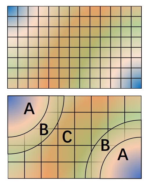
Fig. 3 Regular and hybrid orbital representation. Regular B-spline representation (left panel) contains only one region and a sufficiently fine mesh to resolve orbitals near the nucleus. The hybrid orbital representation (right panel) contains near nucleus regions (A) where spherical harmonics and radial functions are used, buffers or interpolation regions (B), and an interstitial region (C) where a coarse B-spline mesh is used.
Orbitals within region A are computed as
Orbitals in region C are computed as the regular B-spline basis described in Spline basis sets above. The region B interpolates between A and C as
To enable hybrid orbital representation, the input XML needs to see the tag hybridrep="yes" shown in Listing 6.
<determinantset type="bspline" source="i" href="pwscf.h5"
              tilematrix="1 1 3 1 2 -1 -2 1 0" twistnum="-1" gpu="yes" meshfactor="0.8"
              twist="0  0  0" precision="single" hybridrep="yes">
  ...
</determinantset>
Second, the information describing the atomic regions is required in the particle set, shown in Listing 7.
<group name="Ni">
  <parameter name="charge">          18 </parameter>
  <parameter name="valence">         18 </parameter>
  <parameter name="atomicnumber" >   28 </parameter>
  <parameter name="cutoff_radius" > 1.6 </parameter>
  <parameter name="inner_cutoff" >  1.3 </parameter>
  <parameter name="lmax" >            5 </parameter>
  <parameter name="spline_radius" > 1.8 </parameter>
  <parameter name="spline_npoints">  91 </parameter>
</group>
The parameters specific to hybrid representation are listed as
attrib element
Attribute:
Name |
Datatype |
Values |
Default |
Description |
|---|---|---|---|---|
|
Real |
>=0.0 |
None |
Cutoff radius for B/C boundary |
|
Integer |
>=0 |
None |
Largest angular channel |
|
Real |
>=0.0 |
Dep. |
Cutoff radius for A/B boundary |
|
Real |
>0.0 |
Dep. |
Radial function radius used in spine |
|
Integer |
>0 |
Dep. |
Number of spline knots |
cutoff_radiusis required for every species. If a species is intended to not be covered by atomic regions, setting the value 0.0 will put default values for all the reset parameters. A good value is usually a bit larger than the core radius listed in the pseudopotential file. After a parametric scan, pick the one from the flat energy region with the smallest variance.lmaxis required ifcutoff_radius\(>\) 0.0. This value usually needs to be at least the highest angular momentum plus 2.inner_cutoffis optional and set ascutoff_radius\(-0.3\) by default, which is fine in most cases.spline_radiusandspline_npointsare optional. By default, they are calculated based oncutoff_radiusand a grid displacement 0.02 bohr. If users prefer inputing them, it is required thatcutoff_radius<=spline_radius\(-\) 2 \(\times\)spline_radius/(spline_npoints\(-\) 1).
In addition, the hybrid orbital representation allows extra optimization to speed up the nonlocal pseudopotential evaluation using the batched algorithm listed in Pseudopotentials.
Plane-wave basis sets
Homogeneous electron gas
The interacting Fermi liquid has its own special determinantset for filling up a
Fermi surface. The shell number can be specified separately for both spin-up and spin-down.
This determines how many electrons to include of each time; only closed shells are currently
implemented. The shells are filled according to the rules of a square box; if other lattice
vectors are used, the electrons might not fill up a complete shell.
This following example can also be used for Helium simulations by specifying the proper pair interaction in the Hamiltonian section.
<qmcsystem>
<simulationcell name="global">
<parameter name="rs" pol="0" condition="74">6.5</parameter>
<parameter name="bconds">p p p</parameter>
<parameter name="LR_dim_cutoff">15</parameter>
</simulationcell>
<particleset name="e" random="yes">
<group name="u" size="37">
<parameter name="charge">-1</parameter>
<parameter name="mass">1</parameter>
</group>
<group name="d" size="37">
<parameter name="charge">-1</parameter>
<parameter name="mass">1</parameter>
</group>
</particleset>
</qmcsystem>
<qmcsystem>
  <wavefunction name="psi0" target="e">
    <determinantset type="electron-gas" shell="7" shell2="7" randomize="true">
  </determinantset>
    <jastrow name="J2" type="Two-Body" function="Bspline" print="no">
      <correlation speciesA="u" speciesB="u" size="8" cusp="0">
        <coefficients id="uu" type="Array" optimize="yes">
      </correlation>
      <correlation speciesA="u" speciesB="d" size="8" cusp="0">
        <coefficients id="ud" type="Array" optimize="yes">
      </correlation>
    </jastrow>
Jastrow Factors
Jastrow factors are among the simplest and most effective ways of including dynamical correlation in the trial many body wavefunction. The resulting many body wavefunction is expressed as the product of an antisymmetric (in the case of Fermions) or symmetric (for Bosons) part and a correlating Jastrow factor like so:
In this section we will detail the types and forms of Jastrow factor used
in QMCPACK. Note that each type of Jastrow factor needs to be specified using
its own individual jastrow XML element. For this reason, we have repeated the
specification of the jastrow tag in each section, with specialization for the
options available for that given type of Jastrow.
One-body Jastrow functions
The one-body Jastrow factor is a form that allows for the direct inclusion of correlations between particles that are included in the wavefunction with particles that are not explicitly part of it. The most common example of this are correlations between electrons and ions.
The Jastrow function is specified within a wavefunction element
and must contain one or more correlation elements specifying
additional parameters as well as the actual coefficients.
Example use cases gives examples of the typical nesting of
jastrow, correlation, and coefficient elements.
Input Specification
Jastrow element:
name
datatype
values
defaults
description
name
text
(required)
Unique name for this Jastrow function
type
text
One-body
(required)
Define a one-body function
function
text
Bspline
(required)
BSpline Jastrow
text
pade2
Pade form
text
…
…
source
text
name
(required)
Name of attribute of classical particle set
text
yes / no
yes
Jastrow factor printed in external file?
elements
Correlation
Contents
(None)
To be more concrete, the one-body Jastrow factors used to describe correlations between electrons and ions take the form below:
where I runs over all of the ions in the calculation, i runs over the electrons and \(u_{ab}\) describes the functional form of the correlation between them. Many different forms of \(u_{ab}\) are implemented in QMCPACK. We will detail two of the most common ones below.
Spline form
The one-body spline Jastrow function is the most commonly used one-body Jastrow for solids. This form was first described and used in [EKCS12]. Here \(u_{ab}\) is an interpolating 1D B-spline (tricublc spline on a linear grid) between zero distance and \(r_{cut}\). In 3D periodic systems the default cutoff distance is the Wigner Seitz cell radius. For other periodicities, including isolated molecules, the \(r_{cut}\) must be specified. The cusp can be set. \(r_i\) and \(R_I\) are most commonly the electron and ion positions, but any particlesets that can provide the needed centers can be used.
Correlation element:
Name
Datatype
Values
Defaults
Description
ElementType
Text
Name
See below
Classical particle target
SpeciesA
Text
Name
See below
Classical particle target
SpeciesB
Text
Name
See below
Quantum species target
Size
Integer
\(> 0\)
(Required)
Number of coefficients
Rcut
Real
\(> 0\)
See below
Distance at which the correlation goes to 0
Cusp
Real
\(\ge 0\)
0
Value for use in Kato cusp condition
Spin
Text
Yes or no
No
Spin dependent Jastrow factor
Elements
Coefficients
Contents
(None)
Additional information:
elementType, speciesA, speciesB, spinFor a spin-independent Jastrow factor (spin = “no”), elementType should be the name of the group of ions in the classical particleset to which the quantum particles should be correlated. For a spin-dependent Jastrow factor (spin = “yes”), set speciesA to the group name in the classical particleset and speciesB to the group name in the quantum particleset.
rcutThe cutoff distance for the function in atomic units (bohr). For 3D fully periodic systems, this parameter is optional, and a default of the Wigner Seitz cell radius is used. Otherwise this parameter is required.
cuspThe one-body Jastrow factor can be used to make the wavefunction satisfy the electron-ion cusp condition :cite:
kato. In this case, the derivative of the Jastrow factor as the electron approaches the nucleus will be given by
Note that if the antisymmetric part of the wavefunction satisfies the electron-ion cusp condition (for instance by using single-particle orbitals that respect the cusp condition) or if a nondivergent pseudopotential is used, the Jastrow should be cuspless at the nucleus and this value should be kept at its default of 0.
Coefficients element:
Name
Datatype
Values
Defaults
Description
Id
Text
(Required)
Unique identifier
Type
Text
Array
(Required)
Optimize
Text
Yes or no
Yes
if no, values are fixed in optimizations
Elements
(None)
Contents
(No name)
Real array
Zeros
Jastrow coefficients
Example use cases
Specify a spin-independent function with four parameters. Because rcut is not specified, the default cutoff of the Wigner Seitz cell radius is used; this Jastrow must be used with a 3D periodic system such as a bulk solid. The name of the particleset holding the ionic positions is “i.”
<jastrow name="J1" type="One-Body" function="Bspline" print="yes" source="i">
 <correlation elementType="C" cusp="0.0" size="4">
   <coefficients id="C" type="Array"> 0  0  0  0  </coefficients>
 </correlation>
</jastrow>
Specify a spin-dependent function with seven up-spin and seven down-spin parameters. The cutoff distance is set to 6 atomic units. Note here that the particleset holding the ions is labeled as ion0 rather than “i,” as in the other example. Also in this case, the ion is lithium with a coulomb potential, so the cusp condition is satisfied by setting cusp=”d.”
<jastrow name="J1" type="One-Body" function="Bspline" source="ion0" spin="yes">
  <correlation speciesA="Li" speciesB="u" size="7" rcut="6">
    <coefficients id="eLiu" cusp="3.0" type="Array">
    0.0 0.0 0.0 0.0 0.0 0.0 0.0
    </coefficients>
  </correlation>
  <correlation speciesA="C" speciesB="d" size="7" rcut="6">
    <coefficients id="eLid" cusp="3.0" type="Array">
    0.0 0.0 0.0 0.0 0.0 0.0 0.0
    </coefficients>
  </correlation>
</jastrow>
Pade form
Although the spline Jastrow factor is the most flexible and most commonly used form implemented in QMCPACK, there are times where its flexibility can make it difficult to optimize. As an example, a spline Jastrow with a very large cutoff can be difficult to optimize for isolated systems such as molecules because of the small number of samples present in the tail of the function. In such cases, a simpler functional form might be advantageous. The second-order Pade Jastrow factor, given in (11), is a good choice in such cases.
Unlike the spline Jastrow factor, which includes a cutoff, this form has an infinite range and will be applied to every particle pair (subject to the minimum image convention). It also is a cuspless Jastrow factor, so it should be used either in combination with a single particle basis set that contains the proper cusp or with a smooth pseudopotential.
Correlation element:
Name
Datatype
Values
Defaults
Description
ElementType
Text
Name
See below
Classical particle target
Elements
Coefficients
Contents
(None)
Parameter element:
Name
Datatype
Values
Defaults
Description
Id
String
Name
(Required)
Name for variable
Name
String
A or B or C
(Required)
See (11)
Optimize
Text
Yes or no
Yes
If no, values are fixed in optimizations
Elements
(None)
Contents
(No name)
Real
Parameter value
(Required)
Jastrow coefficients
Example use case
Specify a spin-independent function with independent Jastrow factors for two different species (Li and H). The name of the particleset holding the ionic positions is “i.”
<jastrow name="J1" function="pade2" type="One-Body" print="yes" source="i">
  <correlation elementType="Li">
    <var id="LiA" name="A">  0.34 </var>
    <var id="LiB" name="B"> 12.78 </var>
    <var id="LiC" name="C">  1.62 </var>
  </correlation>
  <correlation elementType="H"">
    <var id="HA" name="A">  0.14 </var>
    <var id="HB" name="B"> 6.88 </var>
    <var id="HC" name="C"> 0.237 </var>
  </correlation>
</jastrow>
Short Range Cusp Form
The idea behind this functor is to encode nuclear cusps and other details at very short range around a nucleus in the region that the Gaussian orbitals of quantum chemistry are not capable of describing correctly. The functor is kept short ranged, because outside this small region, quantum chemistry orbital expansions are already capable of taking on the correct shapes. Unlike a pre-computed cusp correction, this optimizable functor can respond to changes in the wave function during VMC optimization. The functor’s form is
in which \(R_0\) acts as a soft cutoff radius (\(u(r)\) decays to zero quickly beyond roughly this distance) and \(A\) determines the cusp condition.
The simple exponential decay is modified by the \(N\) coefficients \(B_k\) that define an expansion in sigmoidal functions, thus adding detailed structure in a short-ranged region around a nucleus while maintaining the correct cusp condition at the nucleus. Note that sigmoidal functions are used instead of, say, a bare polynomial expansion, as they trend to unity past the soft cutoff radius and so interfere less with the exponential decay that keeps the functor short ranged. Although \(A\), \(R_0\), and the \(B_k\) coefficients can all be optimized as variational parameters, \(A\) will typically be fixed as the desired cusp condition is known.
To specify this one-body Jastrow factor, use an input section like the following.
<jastrow name="J1Cusps" type="One-Body" function="shortrangecusp" source="ion0" print="yes">
  <correlation rcut="6" cusp="3" elementType="Li">
    <var id="LiCuspR0" name="R0" optimize="yes"> 0.06 </var>
    <coefficients id="LiCuspB" type="Array" optimize="yes">
      0 0 0 0 0 0 0 0 0 0
    </coefficients>
  </correlation>
  <correlation rcut="6" cusp="1" elementType="H">
    <var id="HCuspR0" name="R0" optimize="yes"> 0.2 </var>
    <coefficients id="HCuspB" type="Array" optimize="yes">
      0 0 0 0 0 0 0 0 0 0
    </coefficients>
  </correlation>
</jastrow>
Here “rcut” is specified as the range beyond which the functor is assumed to be zero. The value of \(A\) can either be specified via the “cusp” option as shown above, in which case its optimization is disabled, or through its own “var” line as for \(R_0\), in which case it can be specified as either optimizable (“yes”) or not (“no”). The coefficients \(B_k\) are specified via the “coefficients” section, with the length \(N\) of the expansion determined automatically based on the length of the array.
Note that this one-body Jastrow form can (and probably should) be used in conjunction with a longer ranged one-body Jastrow, such as a spline form. Be sure to set the longer-ranged Jastrow to be cusp-free!
Two-body Jastrow functions
The two-body Jastrow factor is a form that allows for the explicit inclusion of dynamic correlation between two particles included in the wavefunction. It is almost always given in a spin dependent form so as to satisfy the Kato cusp condition between electrons of different spins [Kat51].
The two body Jastrow function is specified within a wavefunction element
and must contain one or more correlation elements specifying additional parameters
as well as the actual coefficients. Example use cases gives
examples of the typical nesting of jastrow, correlation and
coefficient elements.
Input Specification
Jastrow element:
name
datatype
values
defaults
description
name
text
(required)
Unique name for this Jastrow function
type
text
Two-body
(required)
Define a one-body function
function
text
Bspline
(required)
BSpline Jastrow
text
yes / no
yes
Jastrow factor printed in external file?
elements
Correlation
Contents
(None)
The two-body Jastrow factors used to describe correlations between electrons take the form
The most commonly used form of two body Jastrow factor supported by the code is a splined Jastrow factor, with many similarities to the one body spline Jastrow.
Spline form
The two-body spline Jastrow function is the most commonly used two-body Jastrow for solids. This form was first described and used in [EKCS12]. Here \(u_{ab}\) is an interpolating 1D B-spline (tricublc spline on a linear grid) between zero distance and \(r_{cut}\). In 3D periodic systems, the default cutoff distance is the Wigner Seitz cell radius. For other periodicities, including isolated molecules, the \(r_{cut}\) must be specified. \(r_i\) and \(r_j\) are typically electron positions. The cusp condition as \(r_i\) approaches \(r_j\) is set by the relative spin of the electrons.
Correlation element:
Name
Datatype
Values
Defaults
Description
SpeciesA
Text
U or d
(Required)
Quantum species target
SpeciesB
Text
U or d
(Required)
Quantum species target
Size
Integer
\(> 0\)
(Required)
Number of coefficients
Rcut
Real
\(> 0\)
See below
Distance at which the correlation goes to 0
Spin
Text
Yes or no
No
Spin-dependent Jastrow factor
Elements
Coefficients
Contents
(None)
Additional information:
speciesA, speciesBThe scale function u(r) is defined for species pairs uu and ud. There is no need to define ud or dd since uu=dd and ud=du. The cusp condition is computed internally based on the charge of the quantum particles.
Coefficients element:
Name
Datatype
Values
Defaults
Description
Id
Text
(Required)
Unique identifier
Type
Text
Array
(Required)
Optimize
Text
Yes or no
Yes
If no, values are fixed in optimizations
Elements
(None)
Contents
(No name)
Real array
Zeros
Jastrow coefficients
Example use cases
Specify a spin-dependent function with four parameters for each channel. In this case, the cusp is set at a radius of 4.0 bohr (rather than to the default of the Wigner Seitz cell radius). Also, in this example, the coefficients are set to not be optimized during an optimization step.
<jastrow name="J2" type="Two-Body" function="Bspline" print="yes">
  <correlation speciesA="u" speciesB="u" size="8" rcut="4.0">
    <coefficients id="uu" type="Array" optimize="no"> 0.2309049836 0.1312646071 0.05464141356 0.01306231516</coefficients>
  </correlation>
  <correlation speciesA="u" speciesB="d" size="8" rcut="4.0">
    <coefficients id="ud" type="Array" optimize="no"> 0.4351561096 0.2377951747 0.1129144262 0.0356789236</coefficients>
  </correlation>
</jastrow>
User defined functional form
To aid in implementing different forms for \(u_{ab}(r)\), there is a
script that uses a symbolic expression to generate the appropriate code
(with spatial and parameter derivatives). The script is located in
src/QMCWaveFunctions/Jastrow/codegen/user_jastrow.py. The script
requires Sympy (www.sympy.org) for symbolic mathematics and code
generation.
To use the script, modify it to specify the functional form and a list of variational parameters. Optionally, there may be fixed parameters - ones that are specified in the input file, but are not part of the variational optimization. Also one symbol may be specified that accepts a cusp value in order to satisfy the cusp condition. There are several example forms in the script. The default form is the simple Padé.
Once the functional form and parameters are specified in the script, run
the script from the codegen directory and recompile QMCPACK. The
main output of the script is the file
src/QMCWaveFunctions/Jastrow/UserFunctor.h. The script also prints
information to the screen, and one section is a sample XML input block
containing all the parameters.
There is a unit test in
src/QMCWaveFunctions/test/test_user_jastrow.cpp to perform some
minimal testing of the Jastrow factor. The unit test will need updating
to properly test new functional forms. Most of the changes relate to the
number and name of variational parameters.
Jastrow element:
name
datatype
values
defaults
description
name
text
(required)
Unique name for this Jastrow function
type
text
One-body
(required)
Define a one-body function
Two-body
(required)
Define a two-body function
function
text
user
(required)
User-defined functor
See other parameters as appropriate for one or two-body functions
elements
Correlation
Contents
(None)
Long-ranged Jastrow factors
While short-ranged Jastrow factors capture the majority of the benefit for minimizing the total energy and the energy variance, long-ranged Jastrow factors are important to accurately reproduce the short-ranged (long wavelength) behavior of quantities such as the static structure factor, and are therefore essential for modern accurate finite size corrections in periodic systems.
Below two types of long-ranged Jastrow factors are described. The first (the k-space Jastrow) is simply an expansion of the one and/or two body correlation functions in plane waves, with the coefficients comprising the optimizable parameters. The second type have few variational parameters and use the optimized breakup method of Natoli and Ceperley [NC95] (the Yukawa and Gaskell RPA Jastrows).
Long-ranged Jastrow: k-space Jastrow
The k-space Jastrow introduces explicit long-ranged dependence commensurate with the periodic supercell. This Jastrow is to be used in periodic boundary conditions only.
The input for the k-space Jastrow fuses both one and two-body forms into a single element and so they are discussed together here. The one- and two-body terms in the k-Space Jastrow have the form:
Here \(\rho_G\) is the Fourier transform of the instantaneous electron density:
and \(\rho_G^I\) has the same form, but for the fixed ions. In both cases the coefficients are restricted to be real, though in general the coefficients for the one-body term need not be. See Feature: Reciprocal-space Jastrow factors for more detail.
Input for the k-space Jastrow follows the familar nesting of jastrow-correlation-coefficients elements, with attributes unique to the k-space Jastrow at the correlation input level.
jastrow type=kSpace element:
parent elements:
wavefunctionchild elements:
correlation
attributes:
Name
Datatype
Values
Default
Description
type\(^r\)text
kSpace
must be kSpace
name\(^r\)text
anything
0
Unique name for Jastrow
source\(^r\)text
particleset.nameIon particleset name
correlation element:
parent elements:
jastrow type=kSpacechild elements:
coefficients
attributes:
Name
Datatype
Values
Default
Description
type\(^r\)text
One-body, Two-Body
Must be One-body/Two-body
kc\(^r\)real
kc \(\ge\) 0
0.0
k-space cutoff in a.u.
symmetry\(^o\)text
crystal,isotropic,none
crystal
symmetry of coefficients
spinDependent\(^o\)boolean
yes,no
no
No current function
coefficients element:
parent elements:
correlationchild elements:
None
attributes:
Name
Datatype
Values
Default
Description
id\(^r\)text
anything
cG1/cG2
Label for coeffs
type\(^r\)text
Array0
Must be Array
body text: The body text is a list of real values for the parameters.
Additional information:
It is normal to provide no coefficients as an initial guess. The number of coefficients will be automatically calculated according to the k-space cutoff + symmetry and set to zero.
Providing an incorrect number of parameters also results in all parameters being set to zero.
There is currently no way to turn optimization on/off for the k-space Jastrow. The coefficients are always optimized.
Spin dependence is currently not implemented for this Jastrow.
kc: Parameters with G vectors magnitudes less thankcare included in the Jastrow. Ifkcis zero, it is the same as excluding the k-space term.symmetry=crystal: Impose crystal symmetry on coefficients according to the structure factor.symmetry=isotropic: Impose spherical symmetry on coefficients according to G-vector magnitude.symmetry=none: Impose no symmetry on the coefficients.
<jastrow type="kSpace" name="Jk" source="ion0">
  <correlation kc="4.0" type="One-Body" symmetry="cystal">
    <coefficients id="cG1" type="Array">
    </coefficients>
  </correlation>
  <correlation kc="4.0" type="Two-Body" symmetry="crystal">
    <coefficients id="cG2" type="Array">
    </coefficients>
 </correlation>
</jastrow>
<jastrow type="kSpace" name="Jk" source="ion0">
   <correlation kc="4.0" type="One-Body" symmetry="crystal">
      <coefficients id="cG1" type="Array">
      </coefficients>
   </correlation>
</jastrow>
<jastrow type="kSpace" name="Jk" source="ion0">
   <correlation kc="4.0" type="Two-Body" symmetry="crystal">
      <coefficients id="cG2" type="Array">
      </coefficients>
   </correlation>
</jastrow>
Long-ranged Jastrows: Gaskell RPA and Yukawa forms
NOTE: The Yukawa and RPA Jastrows do not work at present and are currently being revived. Please contact the developers if you are interested in using them.
The exact Jastrow correlation functions contain terms which have a form similar to the Coulomb pair potential. In periodic systems the Coulomb potential is replaced by an Ewald summation of the bare potential over all periodic image cells. This sum is often handled by the optimized breakup method [NC95] and this same approach is applied to the long-ranged Jastrow factors in QMCPACK.
There are two main long-ranged Jastrow factors of this type implemented in QMCPACK: the Gaskell RPA [Gas61][Gas62] form and the [Cep78] form. Both of these forms were used by Ceperley in early studies of the electron gas [Cep78], but they are also appropriate starting points for general solids.
The Yukawa form is defined in real space. It’s long-range form is formally defined as
with \(u_Y(r)\) given by
In QMCPACK a slightly more restricted form is used:
here “\(r_s\)” is understood to be a variational parameter.
The Gaskell RPA form—which contains correct short/long range limits and minimizes the total energy of the electron gas within the RPA—is defined directly in k-space:
where $v_k$ is the Fourier transform of the Coulomb potential and \(S_0(k)\) is the static structure factor of the non-interacting electron gas:
When written in atomic units, RPA Jastrow implemented in QMCPACK has the form
Here “\(r_s\)” is again a variational parameter and \(k_F\equiv(\tfrac{9\pi}{4r_s^3})^{1/3}\).
For both the Yukawa and Gaskell RPA Jastrows, the default value for \(r_s\) is \(r_s=(\tfrac{3\Omega}{4\pi N_e})^{1/3}\).
jastrow type=Two-Body function=rpa/yukawa element:
parent elements:
wavefunctionchild elements:
correlationattributes:
Name
Datatype
Values
Default
Description
type\(^r\)text
Two-body
Must be two-body
function\(^r\)text
rpa/yukawa
Must be rpa or yukawa
name\(^r\)text
anything
RPA_Jee
Unique name for Jastrow
longrange\(^o\)boolean
yes/no
yes
Use long-range part
shortrange\(^o\)boolean
yes/no
yes
Use short-range part
parameters:
Name
Datatype
Values
Default
Description
rs\(^o\)rs
\(r_s>0\)
\(\tfrac{3\Omega}{4\pi N_e}\)
Avg. elec-elec distance
kc\(^o\)kc
\(k_c>0\)
\(2\left(\tfrac{9\pi}{4}\right)^{1/3}\tfrac{4\pi N_e}{3\Omega}\)
k-space cutoff
<jastrow name=''Jee'' type=''Two-Body'' function=''rpa''>
</jastrow>
Three-body Jastrow functions
Explicit three-body correlations can be included in the wavefunction via the three-body Jastrow factor. The three-body electron-electron-ion correlation function (\(u_{\sigma\sigma'I}\)) currently used in is identical to the one proposed in [DTN04]:
Here \(M_{eI}\) and \(M_{ee}\) are the maximum polynomial orders of the electron-ion and electron-electron distances, respectively, \(\{\gamma_{\ell mn}\}\) are the optimizable parameters (modulo constraints), \(r_c\) is a cutoff radius, and \(r_{ab}\) are the distances between electrons or ions \(a\) and \(b\). i.e. The correlation function is only a function of the interparticle distances and not a more complex function of the particle positions, \(\mathbf{r}\). As indicated by the \(\Theta\) functions, correlations are set to zero beyond a distance of \(r_c/2\) in either of the electron-ion distances and the largest meaningful electron-electron distance is \(r_c\). This is the highest-order Jastrow correlation function currently implemented.
Today, solid state applications of QMCPACK usually utilize one and two-body B-spline Jastrow functions, with calculations on heavier elements often also using the three-body term described above.
Example use case
Here is an example of H2O molecule. After optimizing one and two body Jastrow factors, add the following block in the wavefunction. The coefficients will be filled zero automatically if not given.
<jastrow name="J3" type="eeI" function="polynomial" source="ion0" print="yes">
  <correlation ispecies="O" especies="u" isize="3" esize="3" rcut="10">
    <coefficients id="uuO" type="Array" optimize="yes"> </coefficients>
  </correlation>
  <correlation ispecies="O" especies1="u" especies2="d" isize="3" esize="3" rcut="10">
    <coefficients id="udO" type="Array" optimize="yes"> </coefficients>
  </correlation>
  <correlation ispecies="H" especies="u" isize="3" esize="3" rcut="10">
    <coefficients id="uuH" type="Array" optimize="yes"> </coefficients>
  </correlation>
  <correlation ispecies="H" especies1="u" especies2="d" isize="3" esize="3" rcut="10">
    <coefficients id="udH" type="Array" optimize="yes"> </coefficients>
  </correlation>
</jastrow>
Multideterminant wavefunctions
Multiple schemes to generate a multideterminant wavefunction are possible, from CASSF to full CI or selected CI. The QMCPACK converter can convert MCSCF multideterminant wavefunctions from GAMESS [SBB+93] and CIPSI [EG13] wavefunctions from Quantum Package [Sce17] (QP). Full details of how to run a CIPSI calculation and convert the wavefunction for QMCPACK are given in CIPSI wavefunction interface.
The script utils/determinants_tools.py can be used to generate
useful information about the multideterminant wavefunction. This script takes, as a required argument, the path of an h5 file corresponding to the wavefunction. Used without optional arguments, it prints the number of determinants, the number of CSFs, and a histogram of the excitation degree.
> determinants_tools.py ./tests/molecules/C2_pp/C2.h5
Summary:
excitation degree 0 count: 1
excitation degree 1 count: 6
excitation degree 2 count: 148
excitation degree 3 count: 27
excitation degree 4 count: 20

n_det 202
n_csf 104
If the --verbose argument is used, the script will print each determinant,
the associated CSF, and the excitation degree relative to the first determinant.
> determinants_tools.py -v ./tests/molecules/C2_pp/C2.h5 | head
1
alpha  1111000000000000000000000000000000000000000000000000000000
beta   1111000000000000000000000000000000000000000000000000000000
scf    2222000000000000000000000000000000000000000000000000000000
excitation degree  0

2
alpha  1011100000000000000000000000000000000000000000000000000000
beta   1011100000000000000000000000000000000000000000000000000000
scf    2022200000000000000000000000000000000000000000000000000000
excitation degree  2
Backflow Wavefunctions
One can perturb the nodal surface of a single-Slater/multi-Slater wavefunction through use of a backflow transformation. Specifically, if we have an antisymmetric function \(D(\mathbf{x}_{0\uparrow},\cdots,\mathbf{x}_{N\uparrow}, \mathbf{x}_{0\downarrow},\cdots,\mathbf{x}_{N\downarrow})\), and if \(i_\alpha\) is the \(i\)-th particle of species type \(\alpha\), then the backflow transformation works by making the coordinate transformation \(\mathbf{x}_{i_\alpha} \to \mathbf{x}'_{i_\alpha}\) and evaluating \(D\) at these new “quasiparticle” coordinates. QMCPACK currently supports quasiparticle transformations given by
Here, \(\eta^{\alpha\beta}(|\mathbf{x}_{i_\alpha}-\mathbf{x}_{j_\beta}|)\) is a radially symmetric backflow transformation between species \(\alpha\) and \(\beta\). In QMCPACK, particle \(i_\alpha\) is known as the “target” particle and \(j_\beta\) is known as the “source.” The main types of transformations are so-called one-body terms, which are between an electron and an ion \(\eta^{eI}(|\mathbf{x}_{i_e}-\mathbf{x}_{j_I}|)\) and two-body terms. Two-body terms are distinguished as those between like and opposite spin electrons: \(\eta^{e(\uparrow)e(\uparrow)}(|\mathbf{x}_{i_e(\uparrow)}-\mathbf{x}_{j_e(\uparrow)}|)\) and \(\eta^{e(\uparrow)e(\downarrow)}(|\mathbf{x}_{i_e(\uparrow)}-\mathbf{x}_{j_e(\downarrow)}|)\). Henceforth, we will assume that \(\eta^{e(\uparrow)e(\uparrow)}=\eta^{e(\downarrow)e(\downarrow)}\).
In the following, we explain how to describe general terms such as (24) in a QMCPACK XML file. For specificity, we will consider a particle set consisting of H and He (in that order). This ordering will be important when we build the XML file, so you can find this out either through your specific declaration of <particleset>, by looking at the hdf5 file in the case of plane waves, or by looking at the QMCPACK output file in the section labeled “Summary of QMC systems.”
Input specifications
All backflow declarations occur within a single <backflow> ... </backflow> block. Backflow transformations occur in <transformation> blocks and have the following input parameters:
Transformation element:
Name
Datatype
Values
Default
Description
name
Text
(Required)
Unique name for this Jastrow function.
type
Text
“e-I”
(Required)
Define a one-body backflow transformation.
Text
“e-e”
Define a two-body backflow transformation.
function
Text
B-spline
(Required)
B-spline type transformation (no other types supported).
source
Text
“e” if two body, ion particle set if one body.
Just like one- and two-body jastrows, parameterization of the backflow transformations are specified within the <transformation> blocks by <correlation> blocks. Please refer to Spline form for more information.
Example Use Case
Having specified the general form, we present a general example of one-body and two-body backflow transformations in a hydrogen-helium mixture. The hydrogen and helium ions have independent backflow transformations, as do the like and unlike-spin two-body terms. One caveat is in order: ionic backflow transformations must be listed in the order they appear in the particle set. If in our example, helium is listed first and hydrogen is listed second, the following example would be correct. However, switching backflow declaration to hydrogen first then helium, will result in an error. Outside of this, declaration of one-body blocks and two-body blocks are not sensitive to ordering.
<backflow>
<!--The One-Body term with independent e-He and e-H terms. IN THAT ORDER -->
<transformation name="eIonB" type="e-I" function="Bspline" source="ion0">
    <correlation cusp="0.0" size="8" type="shortrange" init="no" elementType="He" rcut="3.0">
        <coefficients id="eHeC" type="Array" optimize="yes">
            0 0 0 0 0 0 0 0
        </coefficients>
    </correlation>
    <correlation cusp="0.0" size="8" type="shortrange" init="no" elementType="H" rcut="3.0">
        <coefficients id="eHC" type="Array" optimize="yes">
            0 0 0 0 0 0 0 0
        </coefficients>
    </correlation>
</transformation>

<!--The Two-Body Term with Like and Unlike Spins -->
<transformation name="eeB" type="e-e" function="Bspline" >
    <correlation cusp="0.0" size="7" type="shortrange" init="no" speciesA="u" speciesB="u" rcut="1.2">
        <coefficients id="uuB1" type="Array" optimize="yes">
            0 0 0 0 0 0 0
        </coefficients>
    </correlation>
    <correlation cusp="0.0" size="7" type="shortrange" init="no" speciesA="d" speciesB="u" rcut="1.2">
        <coefficients id="udB1" type="Array" optimize="yes">
            0 0 0 0 0 0 0
        </coefficients>
    </correlation>
</transformation>
</backflow>
Currently, backflow works only with single-Slater determinant wavefunctions. When a backflow transformation has been declared, it should be placed within the <determinantset> block, but outside of the <slaterdeterminant> blocks, like so:
<determinantset ... >
    <!--basis set declarations go here, if there are any -->

    <backflow>
        <transformation ...>
          <!--Here is where one and two-body terms are defined -->
         </transformation>
     </backflow>

     <slaterdeterminant>
         <!--Usual determinant definitions -->
     </slaterdeterminant>
 </determinantset>
Optimization Tips
Backflow is notoriously difficult to optimize—it is extremely nonlinear in the variational parameters and moves the nodal surface around. As such, it is likely that a full Jastrow+Backflow optimization with all parameters initialized to zero might not converge in a reasonable time. If you are experiencing this problem, the following pointers are suggested (in no particular order).
Get a good starting guess for \(\Psi_T\):
Try optimizing the Jastrow first without backflow.
Freeze the Jastrow parameters, introduce only the e-e terms in the backflow transformation, and optimize these parameters.
Freeze the e-e backflow parameters, and then optimize the e-I terms.
If difficulty is encountered here, try optimizing each species independently.
Unfreeze all Jastrow, e-e backflow, and e-I backflow parameters, and reoptimize.
Optimizing Backflow Terms
It is possible that the previous prescription might grind to a halt in steps 2 or 3 with the inability to optimize the e-e or e-I backflow transformation independently, especially if it is initialized to zero. One way to get around this is to build a good starting guess for the e-e or e-I backflow terms iteratively as follows:
Start off with a small number of knots initialized to zero. Set \(r_{cut}\) to be small (much smaller than an interatomic distance).
Optimize the backflow function.
If this works, slowly increase \(r_{cut}\) and/or the number of knots.
Repeat steps 2 and 3 until there is no noticeable change in energy or variance of \(\Psi_T\).
Tweaking the Optimization Run
The following modifications are worth a try in the optimization block:
Try setting “useDrift” to “no.” This eliminates the use of wavefunction gradients and force biasing in the VMC algorithm. This could be an issue for poorly optimized wavefunctions with pathological gradients.
Try increasing “exp0” in the optimization block. Larger values of exp0 cause the search directions to more closely follow those predicted by steepest-descent than those by the linear method.
Note that the new adaptive shift optimizer has not yet been tried with backflow wavefunctions. It should perform better than the older optimizers, but a considered optimization process is still recommended.
Gaussian Product Wavefunction
The Gaussian Product wavefunction implements (25)
where \(\vec{R}_i\) is the position of the \(i^{\text{th}}\) quantum particle and \(\vec{R}_i^o\) is its center. \(\sigma_i\) is the width of the Gaussian orbital around center \(i\).
This variational wavefunction enhances single-particle density at chosen spatial locations with adjustable strengths. It is useful whenever such localization is physically relevant yet not captured by other parts of the trial wavefunction. For example, in an electron-ion simulation of a solid, the ions are localized around their crystal lattice sites. This single-particle localization is not captured by the ion-ion Jastrow. Therefore, the addition of this localization term will improve the wavefunction. The simplest use case of this wavefunction is perhaps the quantum harmonic oscillator (please see the “tests/models/sho” folder for examples).
Input specification
Gaussian Product Wavefunction (ionwf):
Name
Datatype
Values
Default
Description
Name
Text
ionwf
(Required)
Unique name for this wavefunction
Width
Floats
1.0 -1
(Required)
Widths of Gaussian orbitals
Source
Text
ion0
(Required)
Name of classical particle set
Additional information:
widthThere must be one width provided for each quantum particle. If a negative width is given, then its corresponding Gaussian orbital is removed. Negative width is useful if one wants to use Gaussian wavefunction for a subset of the quantum particles.sourceThe Gaussian centers must be specified in the form of a classical particle set. This classical particle set is likely the ion positions “ion0,” hence the name “ionwf.” However, arbitrary centers can be defined using a different particle set. Please refer to the examples in “tests/models/sho.”
Example Use Case
<qmcsystem>
  <simulationcell>
    <parameter name="bconds">
          n n n
    </parameter>
  </simulationcell>
  <particleset name="e">
    <group name="u" size="1">
      <parameter name="mass">5.0</parameter>
      <attrib name="position" datatype="posArray" condition="0">
        0.0001 -0.0001 0.0002
      </attrib>
    </group>
  </particleset>
  <particleset name="ion0" size="1">
    <group name="H">
      <attrib name="position" datatype="posArray" condition="0">
        0 0 0
      </attrib>
    </group>
  </particleset>
  <wavefunction target="e" id="psi0">
    <ionwf name="iwf" source="ion0" width="0.8165"/>
  </wavefunction>
  <hamiltonian name="h0" type="generic" target="e">
    <extpot type="HarmonicExt" mass="5.0" energy="0.3"/>
    <estimator type="latticedeviation" name="latdev"
      target="e"    tgroup="u"
      source="ion0" sgroup="H"/>
  </hamiltonian>
</qmcsystem>
- AlfeG04
D. Alfè and M. J. Gillan. An efficient localized basis set for quantum Monte Carlo calculations on condensed matter. Physical Review B, 70(16):161101, 2004.
- Cep78(1,2)
D. Ceperley. Ground state of the fermion one-component plasma: a monte carlo study in two and three dimensions. Phys. Rev. B, 18:3126–3138, October 1978. URL: https://link.aps.org/doi/10.1103/PhysRevB.18.3126, doi:10.1103/PhysRevB.18.3126.
- DTN04
N. D. Drummond, M. D. Towler, and R. J. Needs. Jastrow correlation factor for atoms, molecules, and solids. Physical Review B - Condensed Matter and Materials Physics, 70(23):1–11, 2004. doi:10.1103/PhysRevB.70.235119.
- EG13
M. Caffarel E. Giner, A. Scemama. Using perturbatively selected configuration interaction in quantum monte carlo calculations. Canadian Journal of Chemistry, 91:9, 2013.
- EKCS12(1,2)
Kenneth P. Esler, Jeongnim Kim, David M. Ceperley, and Luke Shulenburger. Accelerating quantum monte carlo simulations of real materials on gpu clusters. Computing in Science and Engineering, 14(1):40–51, 2012. doi:http://doi.ieeecomputersociety.org/10.1109/MCSE.2010.122.
- FWL90
S. Fahy, X. W. Wang, and Steven G. Louie. Variational quantum Monte Carlo nonlocal pseudopotential approach to solids: Formulation and application to diamond, graphite, and silicon. Physical Review B, 42(6):3503–3522, 1990. doi:10.1103/PhysRevB.42.3503.
- Gas61
T Gaskell. The collective treatment of a fermi gas: ii. Proceedings of the Physical Society, 77(6):1182, 1961. URL: http://stacks.iop.org/0370-1328/77/i=6/a=312.
- Gas62
T Gaskell. The collective treatment of many-body systems: iii. Proceedings of the Physical Society, 80(5):1091, 1962. URL: http://stacks.iop.org/0370-1328/80/i=5/a=307.
- Kat51
T Kato. Fundamental properties of hamiltonian operators of the schrodinger type. Transactions of the American Mathematical Society, 70:195–211, 1951.
- LEKS18
Ye Luo, Kenneth P. Esler, Paul R. C. Kent, and Luke Shulenburger. An efficient hybrid orbital representation for quantum monte carlo calculations. The Journal of Chemical Physics, 149(8):084107, 2018.
- LK18
Ye Luo and Jeongnim Kim. An highly efficient delayed update algorithm for evaluating slater determinants in quantum monte carlo. in preparation, ():, 2018.
- MDAzevedoL+17
T. McDaniel, E. F. D’Azevedo, Y. W. Li, K. Wong, and P. R. C. Kent. Delayed slater determinant update algorithms for high efficiency quantum monte carlo. The Journal of Chemical Physics, 147(17):174107, November 2017. doi:10.1063/1.4998616.
- NC95(1,2)
Vincent Natoli and David M. Ceperley. An optimized method for treating long-range potentials. Journal of Computational Physics, 117(1):171 – 178, 1995. URL: http://www.sciencedirect.com/science/article/pii/S0021999185710546, doi:http://dx.doi.org/10.1006/jcph.1995.1054.
- Sce17
A. Scemamma. Quantum package. https://github.com/LCPQ/quantum_package, 2013–2017.
- SBB+93
Michael W. Schmidt, Kim K. Baldridge, Jerry A. Boatz, Steven T. Elbert, Mark S. Gordon, Jan H. Jensen, Shiro Koseki, Nikita Matsunaga, Kiet A. Nguyen, Shujun Su, Theresa L. Windus, Michel Dupuis, and John A. Montgomery. General atomic and molecular electronic structure system. Journal of Computational Chemistry, 14(11):1347–1363, 1993. URL: http://dx.doi.org/10.1002/jcc.540141112, doi:10.1002/jcc.540141112.