Analyzing QMCPACK data
Using the qmca tool to obtain total energies and related quantities
The qmca tool is the primary means of analyzing scalar-valued data
generated by QMCPACK. Output files that contain scalar-valued data are
*.scalar.dat and *.dmc.dat (see Output Overview for a detailed description of these files).
Quantities that are available for analysis in *.scalar.dat files
include the local energy and its variance, kinetic energy, potential
energy and its components, acceptance ratio, and the average CPU time
spent per block, among others. The *.dmc.dat files provide
information regarding the DMC walker population in addition to the local
energy.
Basic capabilities of qmca include calculating mean values and
associated error bars, processing multiple files at once in batched
fashion, performing twist averaging, plotting mean values by series, and
plotting traces (per block or step) of the underlying data. These
capabilities are explained with accompanying examples in the following
subsections.
To use qmca, installations of Python and NumPy must be present on
the local machine. For graphical plotting, the matplotlib module must
also be available.
An overview of all supported input flags to qmca can be obtained by
typing qmca at the command line with no other inputs (also try
qmca -x for a short list of examples):
>qmca
  no files provided, please see help info below

  Usage: qmca [options] [file(s)]

  Options:
    --version             show program's version number and exit
    -v, --verbose         Print detailed information (default=False).
    -q QUANTITIES, --quantities=QUANTITIES
                          Quantity or list of quantities to analyze.  See names
                          and abbreviations below (default=all).
    -u UNITS, --units=UNITS
                          Desired energy units.  Can be Ha (Hartree), Ry
                          (Rydberg), eV (electron volts), kJ_mol (k.
                          joule/mole), K (Kelvin), J (Joules) (default=Ha).
    -e EQUILIBRATION, --equilibration=EQUILIBRATION
                          Equilibration length in blocks (default=auto).
    -a, --average         Average over files in each series (default=False).
    --save_average        Save averaged data into scalar.dat files.
                          (default=False).
    -w WEIGHTS, --weights=WEIGHTS
                          List of weights for averaging (default=None).
    -j JOIN, --join=JOIN  Join data for a range of series (default=None).
    -b, --reblock         (pending) Use reblocking to calculate statistics
                          (default=False).
    -p, --plot            Plot quantities vs. series (default=False).
    -t, --trace           Plot a trace of quantities (default=False).
    -h, --histogram       (pending) Plot a histogram of quantities
                          (default=False).
    -o, --overlay         Overlay plots (default=False).
    --legend=LEGEND       Placement of legend.  None for no legend, outside for
                          outside legend (default=upper right).
    --noautocorr          Do not calculate autocorrelation. Warning: error bars
                          are no longer valid! (default=False).
    --noac                Alias for --noautocorr (default=False).
    --sac                 Show autocorrelation of sample data (default=False).
    --sv                  Show variance of sample data (default=False).
    --sort                Display output data sorted alphabetically by file name
                          (default=False).
    -i, --image           Save plot files (default prefix: qmca_plot).
    --image-prefix=BASENAME
                          Save plot files with basename prefix
                          (default=None).
    --image-format=FORMAT Output format for saved plots: png, pdf, svg, or eps
                          (default=png).
    -r, --report          (pending) Write a report (default=False).
    -s, --show_options    Print user provided options (default=False).
    -x, --examples        Print examples and exit (default=False).
    --help                Print help information and exit (default=False).
    -d DESIRED_ERROR, --desired_error=DESIRED_ERROR
                          Show number of samples needed for desired error bar
                          (default=none).
    -n PARTICLE_NUMBER, --enlarge_system=PARTICLE_NUMBER
                          Show number of samples needed to maintain error bar on
                          larger system: desired particle number first, current
                          particle number second (default=none)
    --fp=PRECISION        Sets the floating point precision of displayed
                          statistical results.  Must be a floating point format
                          string such as 16.8f, 8.6e, or similar (default=none).
    --nowarn              Suppress warning messages (default=False).
    --average_all         Average over all files, ignoring differences in path
                          (default=False).
    --twist_info=TWIST_INFO
                          Use twist weights in twist_info.dat files or not.
                          Options: "use", "ignore", "require".  "use" means use
                          when present, "ignore" means do not use, "require"
                          means must be used (default=use).
Obtaining a statistically correct mean and error bar
A rough guess at the mean and error bar of the local energy can be
obtained in the following way with qmca:
>qmca -q e qmc.s000.scalar.dat
qmc  series 0  LocalEnergy           =  -45.876150 +/- 0.017688
In this case the VMC energy of an 8-atom cell of diamond is estimated to be \(-45.876(2)\) Hartrees (Ha). This rough guess should not be used for production-level or publication-quality estimates.
To obtain production-level results, the underlying data should first be inspected visually to ensure that all data included in the averaging can be attributed to a distribution sharing the same mean. The first steps of essentially any MC calculation (the “equilibration phase”) do not belong to the equilibrium distribution and should be excluded from estimates of the mean and its error bar.
We can plot a data trace (-t) of the local energy in the
following way:
>qmca -t -q e -e 0 qmc.s000.scalar.dat
The -e 0 part indicates that we do not want any data
to be initially excluded from the calculation of averages. The resulting
plot is shown in Fig. 4. The unphysical
equilibration period is visible on the left side of the plot.
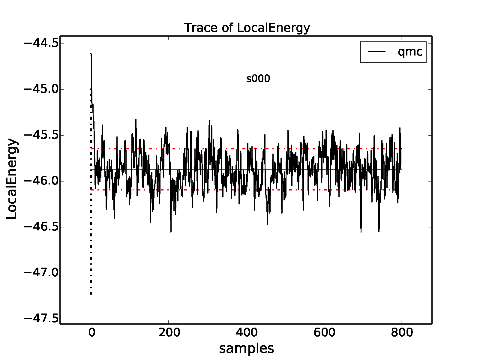
Fig. 4 Trace of the VMC local energy for an 8-atom cell of diamond generated
with qmca. The x-axis (“samples”) refers to the VMC block index in
this case.
Most of the data fluctuates around a well-defined mean (consistent variations around a flat line). This property is important to verify by plotting the trace for each QMC run.
If we exclude none of the equilibration data points, we get an erroneous estimate of \(-45.870(2)\) Ha for the local energy:
>qmca -q e -e 0 qmc.s000.scalar.dat
qmc  series 0  LocalEnergy           =  -45.870071 +/- 0.018072
The equilibration period is typically estimated by eye, though a few conservative values should be checked to ensure that the mean remains unaffected. In this dataset, the equilibration appears to have been reached after 100 or so samples. After excluding the first 100 VMC blocks from the analysis we get
>qmca -q e -e 100 qmc.s000.scalar.dat
qmc  series 0  LocalEnergy           =  -45.877363 +/- 0.017432
This estimate (\(-45.877(2)\) Ha) differs significantly from the
\(-45.870(2)\) Ha figure obtained from the full set of data, but it
agrees with the rough estimate of \(-45.876(2)\) Ha obtained with
the abbreviated command (qmca -q e qmc.s000.scalar.dat). This is
because qmca makes a heuristic guess at the equilibration period and
got it reasonably correct in this case. In many cases, the heuristic
guess fails and should not be relied on for quality results.
We have so far obtained a statistically correct mean. To obtain a statistically correct error bar, it is best to include \(\sim\)100 or more statistically independent samples. An estimate of the number of independent samples can be obtained by considering the autocorrelation time, which is essentially a measure of the number of samples that must be traversed before an uncorrelated/independent sample is reached. We can get an estimate of the autocorrelation time in the following way:
>qmca -q e -e 100 qmc.s000.scalar.dat --sac
qmc  series 0  LocalEnergy           =  -45.877363 +/- 0.017432    4.8
The flag –sac stands for show autocorrelation. In this case,
the autocorrelation estimate is \(4.8\approx 5\) samples. Since the
total run contained 800 samples and we have excluded 100 of them, we can
estimate the number of independent samples as \((800-100)/5=140\).
In this case, the error bar is expected to be estimated reasonably well.
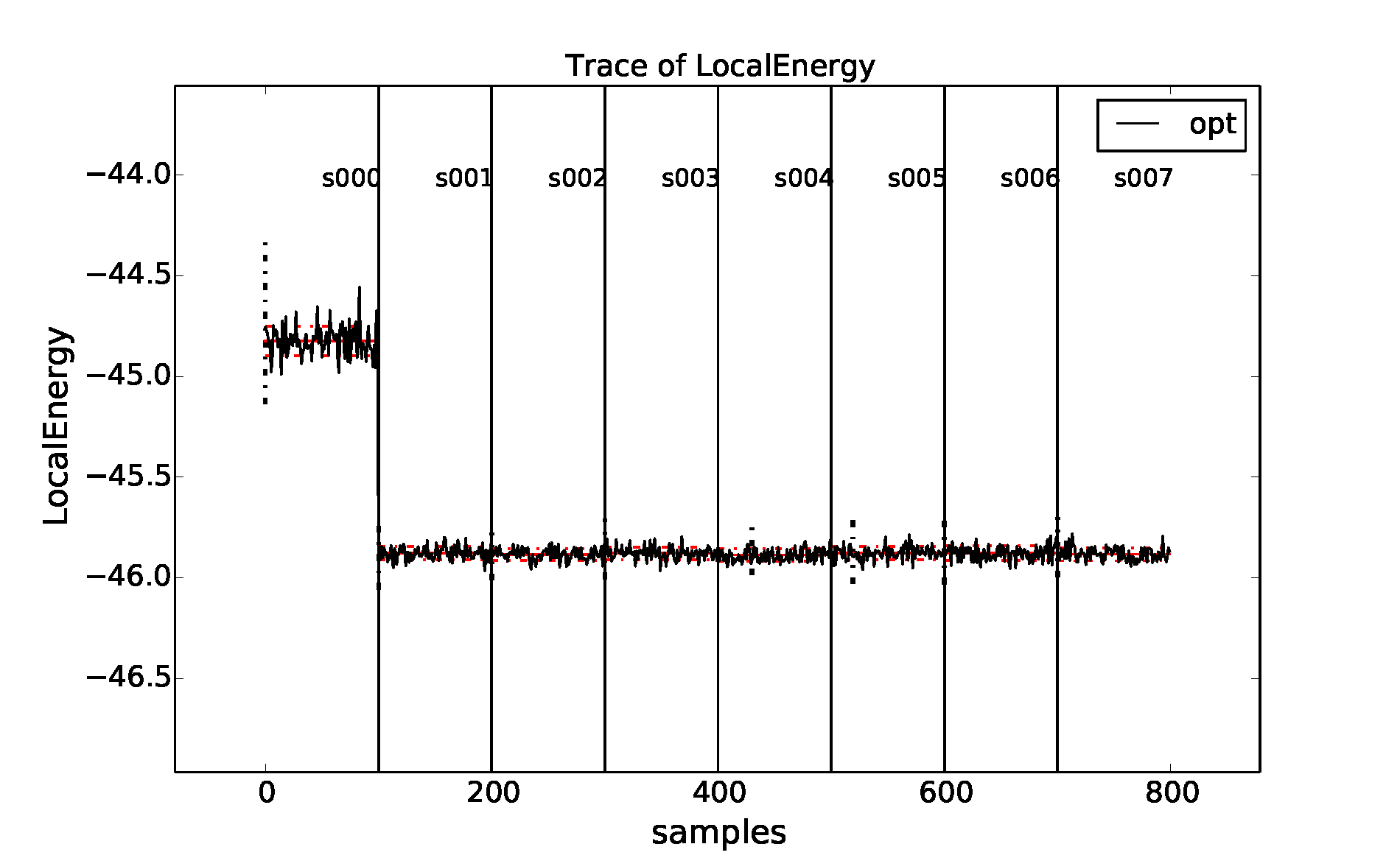
Fig. 5 Trace of the local energy during one- and two-body Jastrow optimizations
for an 8-atom cell of diamond generated with qmca. Data for each
optimization cycle (QMCPACK series) is separated by a vertical black
line.
Keep in mind that the error bar represents the expected range of the mean with a certainty of only \(\sim 70\%\); i.e., it is a one sigma error bar. The actual mean value will lie outside the range indicated by the error bar in 1 out of every 3 runs, and in a set of 20 runs 1 value can be expected to deviate from its estimate by twice the error bar.
Judging wavefunction optimization
Wavefunction optimization is a highly nonlinear and sometimes sensitive process. As such, there is a risk that systematic errors encountered at this stage of the QMC process can be propagated into subsequent (expensive) DMC runs unless they are guarded against with vigilance.
In this section we again consider an 8-atom cell of diamond but now in
the context of Jastrow optimization (one- and two-body terms). In
optimization runs it is often preferable to use a large number of
warmupsteps (\(\sim 100\)) so that equilibration bias does not
propagate into the optimization process. We can check that the added
warm-up has had its intended effect by again checking the local energy
trace:
>qmca -t -q e *scalar*
The resulting plot can be found in Fig. 5. In
this case sufficient warmupsteps were used to exit the equilibration
period before samples were collected and we can proceed without using
the -e option with qmca.
After inspecting the trace, we should inspect the text output from
qmca, now including the total energy and its variance:
>qmca -q ev opt*scalar.dat
                            LocalEnergy               Variance           ratio
opt  series 0  -44.823616 +/- 0.007430   7.054219 +/- 0.041998   0.1574
opt  series 1  -45.877643 +/- 0.003329   1.095362 +/- 0.041154   0.0239
opt  series 2  -45.883191 +/- 0.004149   1.077942 +/- 0.021555   0.0235
opt  series 3  -45.877524 +/- 0.003094   1.074047 +/- 0.010491   0.0234
opt  series 4  -45.886062 +/- 0.003750   1.061707 +/- 0.014459   0.0231
opt  series 5  -45.877668 +/- 0.003475   1.091585 +/- 0.021637   0.0238
opt  series 6  -45.877109 +/- 0.003586   1.069205 +/- 0.009387   0.0233
opt  series 7  -45.882563 +/- 0.004324   1.058771 +/- 0.008651   0.0231
The flags -q ev requested the energy (e) and the variance
(v). For this combination of quantities, a third column (ratio)
is printed containing the ratio of the variance and the absolute value
of the local energy. The variance/energy ratio is an intensive quantity
and is useful to inspect regardless of the system under study.
Successful optimization of molecules and solids of any size generally
result in comparable values for the variance/energy ratio.
The first line of the output (series 0) corresponds to the local
energy and variance of the system without a Jastrow factor (all Jastrow
coefficients were initialized to zero in this case), reflecting the
quality of the orbitals alone. For pseudopotential systems, a
variance/energy ratio \(>0.20\) Ha generally indicates there is a
problem with the input orbitals that needs to be resolved before
performing wavefunction optimization.
The subsequent lines correspond to energies and variances of
intermediate parameterizations of the trial wavefunction during the
optimization process. The output line containing opt series 1, for
example, corresponds to the trial wavefunction parameterized during the
series 0 step (the parameters of this wavefunction would be found in
an output file matching *s000*opt.xml). The first thing to check
about the resulting optimization is again the variance/energy ratio. For
pseudopotential systems, a variance/energy ratio \(<0.03\) Ha is
consistent with a trial wavefunction of production quality, and values
of \(0.01\) Ha are rarely obtainable for standard Slater-Jastrow
wavefunctions. By this metric, all parameterizations obtained for
optimizations performed in series 0-6 are of comparable quality (note
that the quality of the wavefunction obtained during optimization series
7 is effectively unknown).
A good way to further discriminate among the parameterizations is to
plot the energy and variance as a function of series with qmca:
>qmca -p -q ev opt*scalar.dat
The -p option results in plots of means plus error bars
vs. series for all requested quantities.
The resulting plots for the local energy and variance are shown
in Fig. 6. In this case, the resulting energies
and variances are statistically indistinguishable for all optimization
cycles.
A good way to choose the optimal wavefunction for use in DMC is to select the one with the lowest statistically significant energy within the set of optimized wavefunctions with reasonable variance (e.g., among those with a variance/energy ratio \(<0.03\) Ha). For pseudopotential calculations, minimizing according to the total energy is recommended to reduce locality errors in DMC.
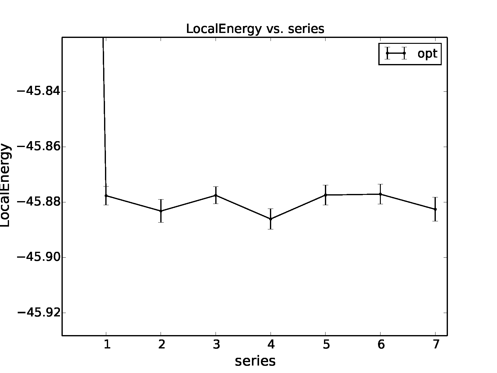
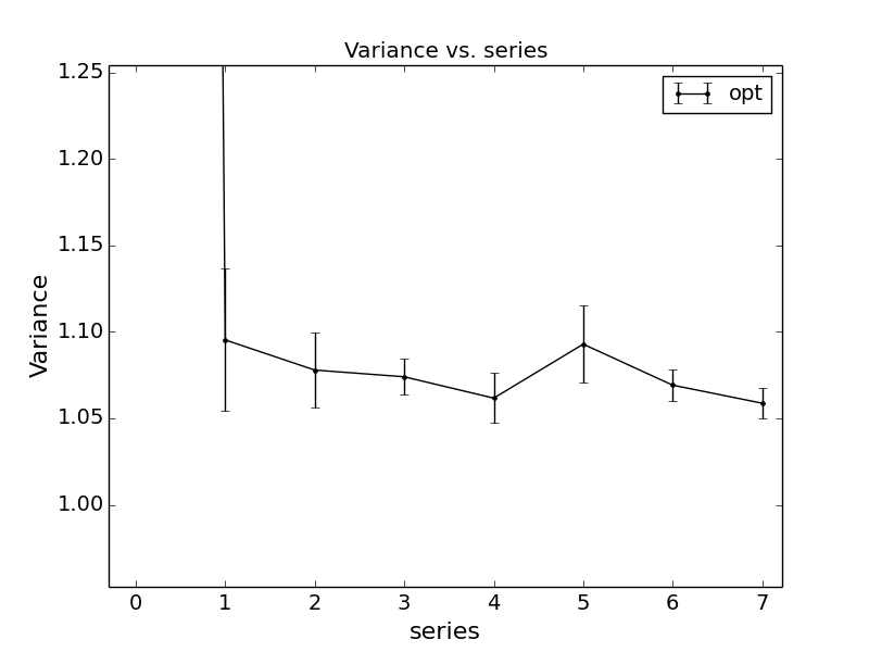
Fig. 6 Energy and variance vs. optimization series for an 8-atom cell of
diamond as plotted by qmca.
Judging diffusion Monte Carlo runs
Judging the quality of the DMC projection process requires more care than is needed in VMC. To reduce bias, a small time step is required in the approximate projector but this also leads to slow equilibration and long autocorrelation times. Systematic errors in the projection process can also arise from statistical fluctuations due to pseudopotentials or from trial wavefunctions with larger-than-necessary variance.
To illustrate the problems that can arise with respect to slow equilibration and long autocorrelation times, we consider the 8-atom diamond system with VMC (\(200\) blocks of \(160\) steps) followed by DMC (\(400\) blocks of \(5\) steps) with a small time step (\(0.002\) Ha\(^{-1}\)). A good first step in assessing the quality of any DMC run is to plot the trace of the local energy:
>qmca -t -q e -e 0 *scalar*
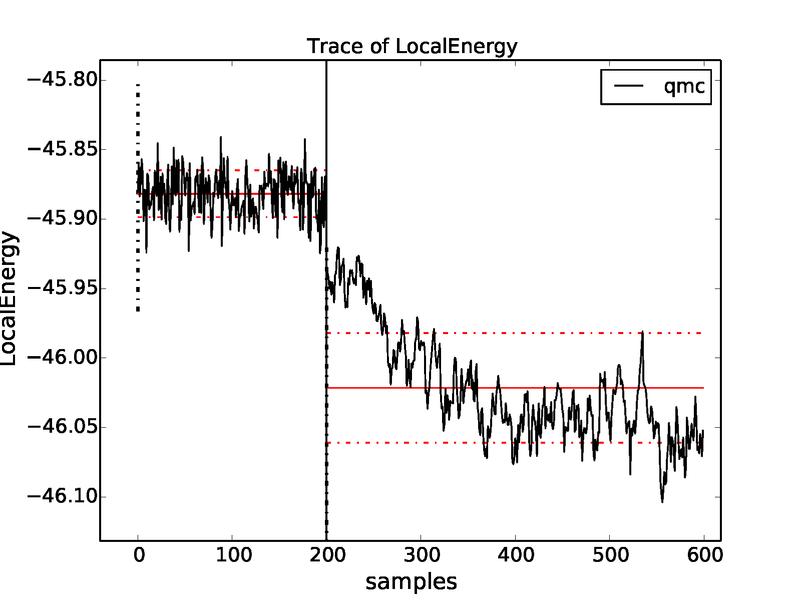
Fig. 7 Trace of the local energy for VMC followed by DMC with a small time step
(\(0.002\) Ha\(^{-1}\)) for an 8-atom cell of diamond
generated with qmca.
The resulting trace plot is shown in Fig. 7. As always, the DMC local energy decreases exponentially away from the VMC value, but in this case it takes a long time to do so. At least half of the DMC run is inefficiently consumed by equilibration. If we are not careful to inspect and remove the transient, the estimated DMC energy will be strongly biased by the transient as shown by the horizontal red line (estimated mean) in the figure. The autocorrelation time is also large (\(\sim 12\) blocks):
>qmca -q e -e 200 --sac *s001.scalar*
qmc  series 1  LocalEnergy           =  -46.045720 +/- 0.004813   11.6
Of the included 200 blocks, fewer than 20 contribute to the estimated error bar, indicating that we cannot trust the reported error bar. This can also be demonstrated directly from the data. If we halve the number of included samples to 100, we expect from Gaussian statistics that the error bar will grow by a factor of \(\sqrt{2}\), but instead we get
>qmca -q e -e 300 *s001.scalar*
qmc  series 1  LocalEnergy           =  -46.048537 +/- 0.009280
which erroneously shows an estimated increase in the error bar by a factor of about 2. Overall, this run is simply too short to gain meaningful information.
Consider the case in which we are interested in the cohesive energy of diamond, and, after having performed a time step study of the cohesive energy, we have found that the energy difference between bulk diamond and atomic carbon converges to our required accuracy with a larger time step of \(0.01\) Ha\(^{-1}\). In a production setting, a small cell could be used to determine the appropriate time step, while a larger cell would subsequently be used to obtain a converged cohesive energy, though for purposes of demonstration we still proceed here with the 8-atom cell. The new time step of \(0.01\) Ha\(^{-1}\) will result in a shorter autocorrelation time than the smaller time step used previously, but we would like to shorten the equilibration time further still. This can be achieved by using a larger time step (say \(0.02\) Ha\(^{-1}\)) in a short intermediate DMC run used to walk down the transient. The rapidly achieved equilibrium with the \(0.02\) Ha\(^{-1}\) time step projector will be much nearer to the \(0.01\) Ha\(^{-1}\) time step we seek than the original VMC equilibrium, so we can expect a shortened secondary equilibration time in the production \(0.01\) Ha\(^{-1}\) time step run. Note that this procedure is fully general, even if having to deal with an even shorter time step (e.g., \(0.002\) Ha\(^{-1}\)) for a particular problem.
We now rerun the previous example but with an intermediate DMC
calculation using \(40\) blocks of \(5\) steps with a time step
of \(0.02\) Ha\(^{-1}\), followed by a production DMC
calculation using \(400\) blocks of \(10\) steps with a time
step of \(0.01\) Ha\(^{-1}\). We again plot the local energy
trace using qmca:
>qmca -t -q e -e 0 *scalar*
with the result shown in Fig. 8. The projection transient has been effectively contained in the short DMC run with a larger time step. As expected, the production run contains only a short equilibration period. Removing the first 20 blocks as a precaution, we obtain an estimate of the total energy in VMC and DMC:
>qmca -q ev -e 20 --sac qmc.*.scalar.dat
                            LocalEnergy               Variance           ratio
qmc  series 0  -45.881042 +/- 0.001283    1.0   1.076726 +/- 0.007013    1.0   0.0235
qmc  series 1  -46.040814 +/- 0.005046    3.9   1.011303 +/- 0.016807    1.1   0.0220
qmc  series 2  -46.032960 +/- 0.002077    5.2   1.014940 +/- 0.002547    1.0   0.0220

Fig. 8 Trace of the local energy for VMC followed by a short intermediate DMC with a large time step (\(0.02\) Ha\(^{-1}\)) and finally a production DMC run with a time step of \(0.01\) Ha\(^{-1}\). Calculations were performed in an 8-atom cell of diamond.
Notice that the variance/energy ratio in DMC (\(0.220\) Ha) is
similar to but slightly smaller than that obtained with VMC
(\(0.235\) Ha). If the DMC variance/energy ratio is ever
significantly larger than with VMC, this is cause to be concerned about
the correctness of the DMC run. Also notice the estimated
autocorrelation time (\(\sim 5\) blocks). This leaves us with an
estimated \(\sim 76\) independent samples, though we should recall
that the autocorrelation time is also a statistical estimate that can be
improved with more data. We can gain a better estimate of the
autocorrelation time by using the *.dmc.dat files, which contain
output data resolved per step rather than per block (there are
\(10\times\) more steps than blocks in this example case):
>qmca -q ev -e 200 --sac qmc.s002.dmc.dat
                            LocalEnergy               Variance           ratio
qmc  series 2  -46.032909 +/- 0.002068   31.2   1.015781 +/- 0.002536    1.4   0.0221
This results in an estimated autocorrelation time of \(\sim 31\) steps, or \(\sim 3\) blocks, indicating that we actually have \(\sim 122\) independent samples, which should be sufficient to obtain a trustworthy error bar. Our final DMC total energy is estimated to be \(-46.0329(2)\) Ha.
Another simulation property that should be explicitly monitored
is the behavior of the DMC walker population. Data regarding the
walker population is contained in the *.dmc.dat files.
In Fig. 9 we show the trace of the DMC
walker population for the current run:
>qmca -t -q nw *dmc.dat
qmc  series 1  NumOfWalkers          =  2056.905405 +/- 8.775527
qmc  series 2  NumOfWalkers          =  2050.164160 +/- 4.954850
Following a DMC run, the walker population should be checked for two qualities: (1) that the population is sufficiently large (a number \(>2,000\) is generally sufficient to reduce population control bias) and (2) that the population fluctuates benignly around its intended target value. In this case the target walker count (provided in the input file) was \(2,048\) and we can confirm from the plot that the population is simply fluctuating around this value. Also, from the text output we have a dynamic population estimate of 2,050(5) walkers. Rapid population reductions or increases—population explosions—are indicative of problems with a run. These issues sometimes result from using a considerably poor wavefunction (see comments regarding variance/energy ratio in the preceding subsections). QMCPACK has internal guards in place that prevent the population from exceeding certain maximum and minimum bounds, so in particularly faulty runs one might see the population “stabilize” to a constant value much larger or smaller than the target. In such cases the cause(s) for the divergent population behavior needs to be investigated and resolved before proceeding further.
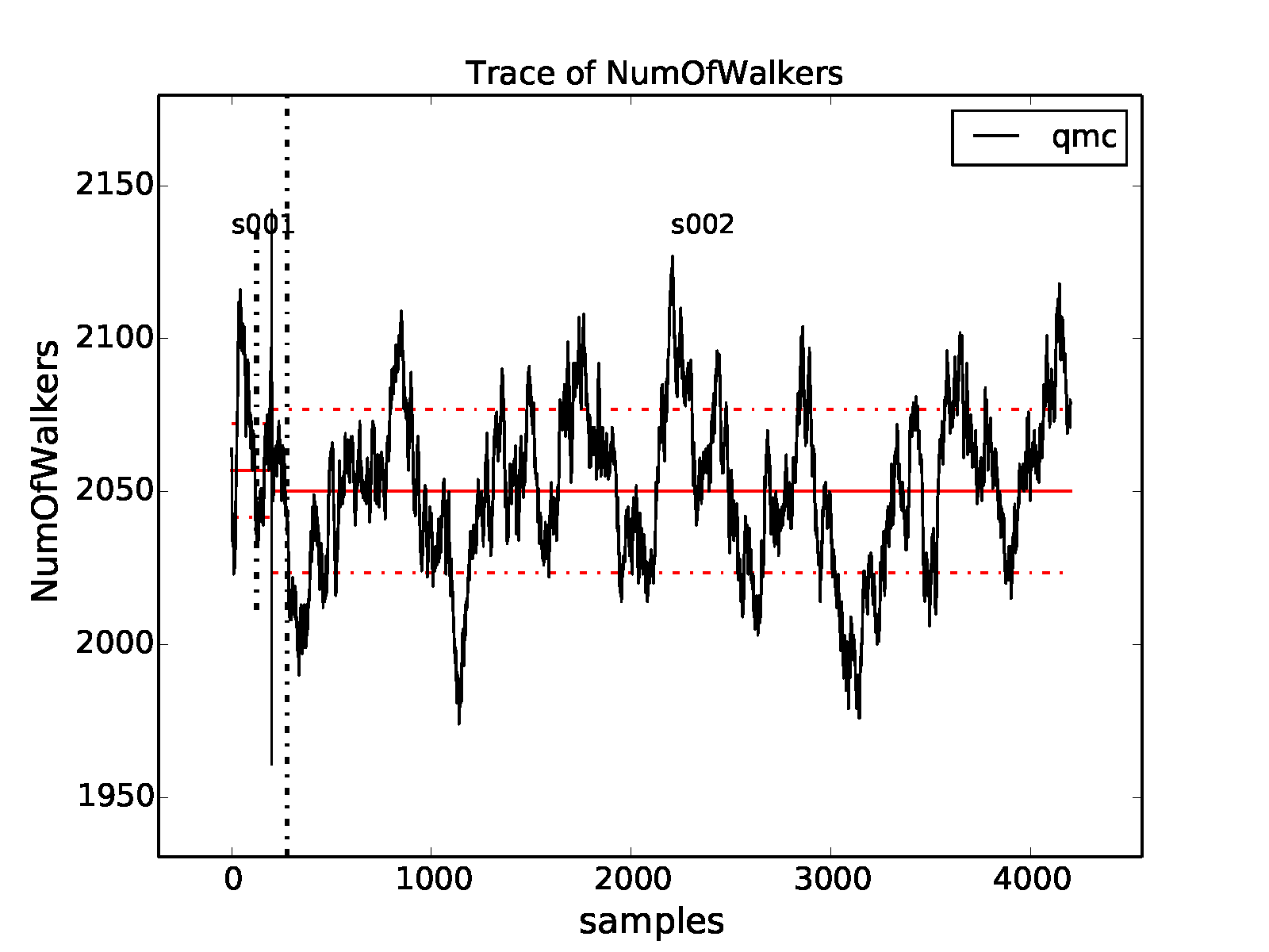
Fig. 9 Trace of the DMC walker population for an 8-atom cell of diamond
obtained with qmca.
Obtaining other quantities
A number of other scalar-valued quantities are available with qmca.
To obtain text output for all quantities available, simply exclude the
-q option used in previous examples. The following example shows
output for a DMC calculation of the 8-atom diamond system from the
scalar.dat file:
>qmca -e 20 qmc.s002.scalar.dat
qmc  series 2
  LocalEnergy           =          -46.0330 +/-           0.0021
  Variance              =            1.0149 +/-           0.0025
  Kinetic               =            33.851 +/-            0.019
  LocalPotential        =           -79.884 +/-            0.020
  ElecElec              =          -11.4483 +/-           0.0083
  LocalECP              =           -22.615 +/-            0.029
  NonLocalECP           =            5.2815 +/-           0.0079
  IonIon                =            -51.10 +/-             0.00
  LocalEnergy_sq        =           2120.05 +/-             0.19
  BlockWeight           =          20514.27 +/-            48.38
  BlockCPU              =            1.4890 +/-           0.0038
  AcceptRatio           =         0.9963954 +/-        0.0000055
  Efficiency            =             71.88 +/-             0.00
  TotalTime             =            565.80 +/-             0.00
  TotalSamples          =           7795421 +/-                0
Similarly, for the dmc.dat file we get
>qmca -e 20 qmc.s002.dmc.dat
qmc  series 2
  LocalEnergy           =          -46.0329 +/-           0.0020
  Variance              =            1.0162 +/-           0.0025
  TotalSamples          =           8201275 +/-                0
  TrialEnergy           =          -46.0343 +/-           0.0023
  DiffEff               =         0.9939150 +/-        0.0000088
  Weight                =           2050.23 +/-             4.82
  NumOfWalkers          =              2050 +/-                5
  LivingFraction        =          0.996427 +/-         0.000021
  AvgSentWalkers        =            0.2625 +/-           0.0011
Any subset of desired quantities can be obtained by using the -q
option with either the full names of the quantities just listed
>qmca -q 'LocalEnergy Kinetic LocalPotential' -e 20 qmc.s002.scalar.dat
qmc  series 2
  LocalEnergy           =          -46.0330 +/-           0.0021
  Kinetic               =            33.851 +/-            0.019
  LocalPotential        =           -79.884 +/-            0.020
or with their corresponding abbreviations.
>qmca -q ekp -e 20 qmc.s002.scalar.dat
qmc  series 2
  LocalEnergy           =          -46.0330 +/-           0.0021
  Kinetic               =            33.851 +/-            0.019
  LocalPotential        =           -79.884 +/-            0.020
Abbreviations for each quantity can be found by typing qmca at the
command line with no other input. This following is a current list:
Abbreviations and full names for quantities:
  ar              = AcceptRatio
  bc              = BlockCPU
  bw              = BlockWeight
  ce              = CorrectedEnergy
  de              = DiffEff
  de_AB           = dLocEne_0_1
  dee_AB          = dElecElec_0_1
  dii_AB          = dIonIon_0_1
  e               = LocalEnergy
  e_A             = LocEne_0
  e_B             = LocEne_1
  ee              = ElecElec
  ee_A            = ElecElec_0
  ee_B            = ElecElec_1
  ee_m            = ElecElec_m
  ee_p            = ElecElec_p
  eff             = Efficiency
  ei_A            = ElecIon_0
  ei_AB           = dElecIon_0_1
  ei_B            = ElecIon_1
  el              = EnergyEstim__nume_real
  fl              = Flux
  fl_A            = Flux_0
  fl_AB           = dFlux_0_1
  fl_B            = Flux_1
  ii              = IonIon
  ii_A            = IonIon_0
  ii_B            = IonIon_1
  k               = Kinetic
  k_A             = Kinetic_0
  k_AB            = dKinetic_0_1
  k_B             = Kinetic_1
  k_m             = Kinetic_m
  k_p             = Kinetic_p
  kc              = KEcorr
  l               = LocalECP
  le2             = LocalEnergy_sq
  mpc             = MPC
  n               = NonLocalECP
  nw              = NumOfWalkers
  p               = LocalPotential
  p_A             = LocPot_0
  p_AB            = dLocPot_0_1
  p_B             = LocPot_1
  p_p             = LocalPotential_pure
  sw              = AvgSentWalkers
  te              = TrialEnergy
  ts              = TotalSamples
  tt              = TotalTime
  v               = Variance
  w               = Weight
  wp_A            = wpsi_0
  wp_B            = wpsi_1
See the output overview for scalar.dat
(The .scalar.dat file) and dmc.dat
(The .dmc.dat file) for more information about
these quantities. The data analysis aspects for these
quantities are essentially the same as for the local
energy as covered in the preceding subsections.
Quantities that do not belong to an equilibrium distribution
(e.g., BlockCPU) are somewhat different, though they
still exhibit statistical fluctuations.
Processing multiple files
Batch file processing is a common use case for qmca. If we consider
an “equation-of-state” calculation involving the 8-atom diamond cell we
have used so far, we might be interested in the total energy for the
various supercell volumes along the trajectory from compression to
expansion. After checking the traces
(qmca -t -q e scale_*/vmc/*scalar*) to settle on a sensible
equilibration cutoff as discussed in the preceding subsections, we can
obtain the total energies all at once:
>qmca -q ev -e 40 scale_*/vmc/*scalar*
                            LocalEnergy               Variance           ratio
scale_0.80/vmc/qmc  series 0 -44.670984 +/- 0.006051  2.542384 +/- 0.019902  0.0569
scale_0.82/vmc/qmc  series 0 -44.982818 +/- 0.005757  2.413011 +/- 0.022626  0.0536
scale_0.84/vmc/qmc  series 0 -45.228257 +/- 0.005374  2.258577 +/- 0.019322  0.0499
scale_0.86/vmc/qmc  series 0 -45.415842 +/- 0.005532  2.204980 +/- 0.052978  0.0486
scale_0.88/vmc/qmc  series 0 -45.570215 +/- 0.004651  2.061374 +/- 0.014359  0.0452
scale_0.90/vmc/qmc  series 0 -45.683684 +/- 0.005009  1.988539 +/- 0.018267  0.0435
scale_0.92/vmc/qmc  series 0 -45.751359 +/- 0.004928  1.913282 +/- 0.013998  0.0418
scale_0.94/vmc/qmc  series 0 -45.791622 +/- 0.005026  1.843704 +/- 0.014460  0.0403
scale_0.96/vmc/qmc  series 0 -45.809256 +/- 0.005053  1.829103 +/- 0.014536  0.0399
scale_0.98/vmc/qmc  series 0 -45.806235 +/- 0.004963  1.775391 +/- 0.015199  0.0388
scale_1.00/vmc/qmc  series 0 -45.783481 +/- 0.005293  1.726869 +/- 0.012001  0.0377
scale_1.02/vmc/qmc  series 0 -45.741655 +/- 0.005627  1.681776 +/- 0.011496  0.0368
scale_1.04/vmc/qmc  series 0 -45.685101 +/- 0.005353  1.682608 +/- 0.015423  0.0368
scale_1.06/vmc/qmc  series 0 -45.615164 +/- 0.005978  1.652155 +/- 0.010945  0.0362
scale_1.08/vmc/qmc  series 0 -45.543037 +/- 0.005191  1.646375 +/- 0.013446  0.0361
scale_1.10/vmc/qmc  series 0 -45.450976 +/- 0.004794  1.707649 +/- 0.048186  0.0376
scale_1.12/vmc/qmc  series 0 -45.371851 +/- 0.005103  1.686997 +/- 0.035920  0.0372
scale_1.14/vmc/qmc  series 0 -45.265490 +/- 0.005311  1.631614 +/- 0.012381  0.0360
scale_1.16/vmc/qmc  series 0 -45.161961 +/- 0.004868  1.656586 +/- 0.014788  0.0367
scale_1.18/vmc/qmc  series 0 -45.062579 +/- 0.005971  1.671998 +/- 0.019942  0.0371
scale_1.20/vmc/qmc  series 0 -44.960477 +/- 0.004888  1.651864 +/- 0.009756  0.0367
In this case, we are using a Jastrow factor optimized only at the
equilibrium geometry (scale_1.00) but with radial cutoffs restricted
to the Wigner-Seitz radius of the most compressed supercell
(scale_0.80) to avoid introducing wavefunction cusps at the cell
boundary (had we tried, QMCPACK would have aborted with a warning in
this case). It is clear that this restricted Jastrow factor is not an
optimal choice because it yields variance/energy ratios between
\(0.036\) and \(0.057\) Ha. This issue is largely a result of
our undersized (8-atom) supercell; larger cells should always be used in
real production calculations.
Batch processing is also possible for multiple quantities. If multiple quantities are requested, an additional line is inserted to separate results from different runs:
>qmca -q 'e bc eff' -e 40 scale_*/vmc/*scalar*
scale_0.80/vmc/qmc  series 0
  LocalEnergy           =          -44.6710 +/-           0.0061
  BlockCPU              =           0.02986 +/-          0.00038
  Efficiency            =          38104.00 +/-             0.00

scale_0.82/vmc/qmc  series 0
  LocalEnergy           =          -44.9828 +/-           0.0058
  BlockCPU              =           0.02826 +/-          0.00013
  Efficiency            =          44483.91 +/-             0.00

scale_0.84/vmc/qmc  series 0
  LocalEnergy           =          -45.2283 +/-           0.0054
  BlockCPU              =           0.02747 +/-          0.00030
  Efficiency            =          52525.12 +/-             0.00

scale_0.86/vmc/qmc  series 0
  LocalEnergy           =          -45.4158 +/-           0.0055
  BlockCPU              =           0.02679 +/-          0.00013
  Efficiency            =          50811.55 +/-             0.00

scale_0.88/vmc/qmc  series 0
  LocalEnergy           =          -45.5702 +/-           0.0047
  BlockCPU              =           0.02598 +/-          0.00015
  Efficiency            =          74148.79 +/-             0.00

scale_0.90/vmc/qmc  series 0
  LocalEnergy           =          -45.6837 +/-           0.0050
  BlockCPU              =           0.02527 +/-          0.00011
  Efficiency            =          65714.98 +/-             0.00

...
Twist averaging
Twist averaging can be performed straightforwardly for any output
quantity listed in Obtaining other quantities with qmca.
We illustrate these capabilities by repeating the 8-atom diamond DMC
runs performed in Section Judging diffusion Monte Carlo runs at 8 real-valued
supercell twist angles (a \(2\times 2\times 2\) Monkhorst-Pack grid
centered at the \(\Gamma\)-point). Data traces for each twist can be
overlapped on the same plot:
>qmca -to -q e -e '30 20 30' *scalar* --legend outside
The -o option requests the plots to be overlapped; otherwise,
8 separate plots would be generated. The
equilibration input -e '30 20 30' cuts out from
the analyzed data the first 30 blocks for series 0 (VMC),
20 blocks for series 1 (intermediate DMC), and 30 blocks for
series 2 (production DMC). The resulting plot is shown in
Fig. 10.
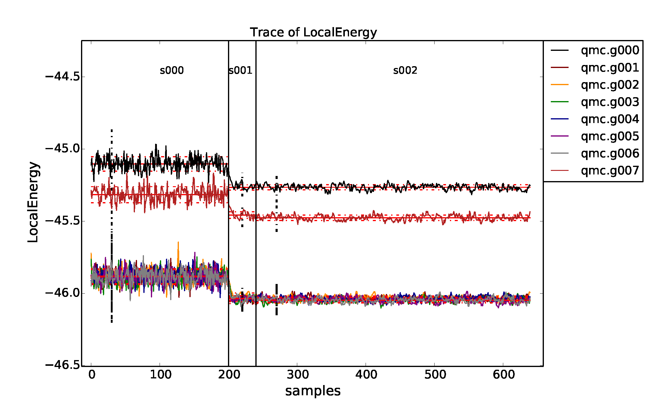
Fig. 10 Overlapped energy traces from VMC to DMC for an 8-supercell diamond
obtained with qmca. Data for each twist appears in a different
color.
Twist averaging is performed by providing the -a
option. If provided on its own, uniform weights are applied
to each twist angle. To obtain a trace plot with twist averaging
enforced, use a command similar to the following:
>qmca -a -t -q e -e '30 20 30' *scalar*
The resulting plot is shown in Fig. 11. As
can be seen from the trace plot, the chosen equilibration lengths are
appropriate, and we proceed to obtain the twist-averaged total energy
from the scalar.dat files
>qmca -a -q ev -e 30 --sac *s002.scalar*
                            LocalEnergy               Variance           ratio
avg  series 2  -45.873369 +/- 0.000753    5.3   1.028751 +/- 0.001056    1.3   0.0224
and also from the dmc.dat files
>qmca -a -q ev -e 300 --sac *s002.dmc*
                          LocalEnergy               Variance           ratio
avg  series 2  -45.873371 +/- 0.000741   30.5   1.028843 +/- 0.000972    1.6   0.0224
yielding a twist-averaged total energy of \(-45.8733(8)\) Ha.
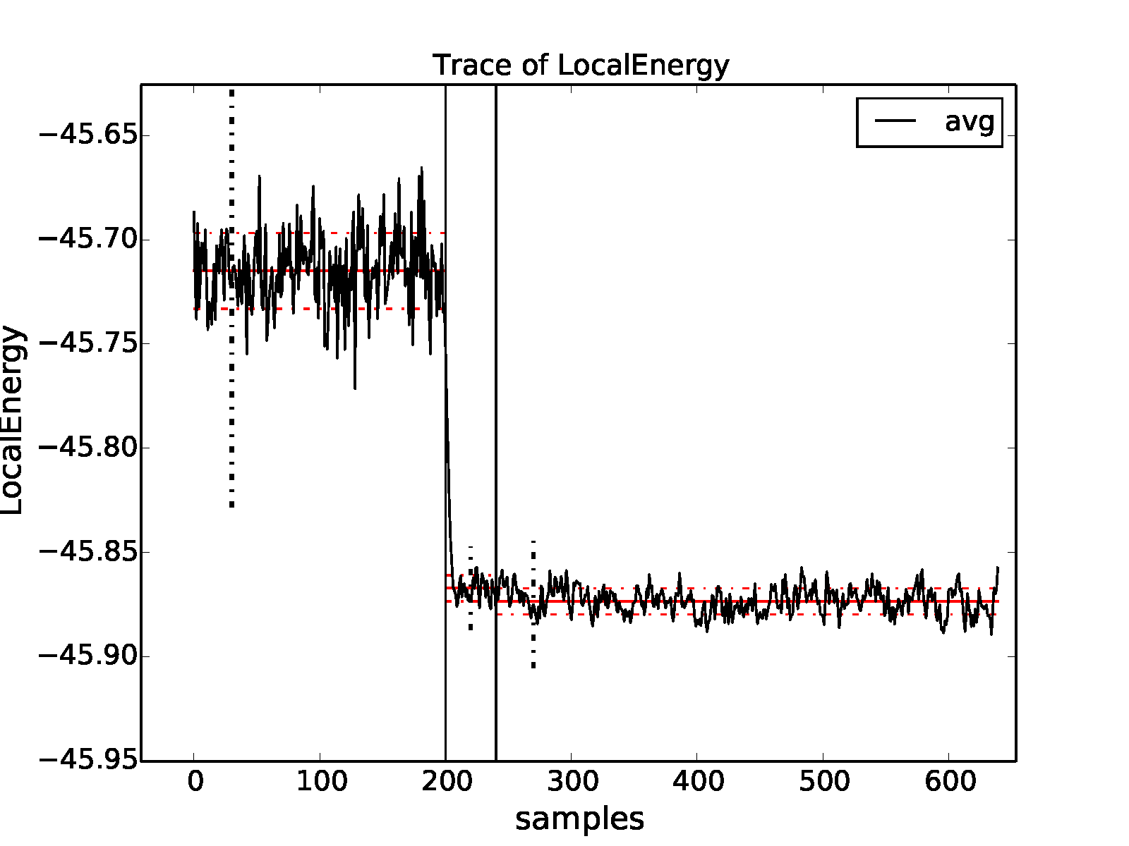
Fig. 11 Twist-averaged energy trace from VMC to DMC for an 8-supercell diamond obtained with qmca.
As can be seen from Fig. 10, some of the twist angles are degenerate. This is seen more clearly in the text output
>qmca -q ev -e 30 *s002.scalar*
                            LocalEnergy               Variance           ratio
qmc.g000  series 2  -45.264510 +/- 0.001942   1.057065 +/- 0.002318   0.0234
qmc.g001  series 2  -46.035511 +/- 0.001806   1.015992 +/- 0.002836   0.0221
qmc.g002  series 2  -46.035410 +/- 0.001538   1.015039 +/- 0.002661   0.0220
qmc.g003  series 2  -46.047285 +/- 0.001898   1.018219 +/- 0.002588   0.0221
qmc.g004  series 2  -46.034225 +/- 0.002539   1.013420 +/- 0.002835   0.0220
qmc.g005  series 2  -46.046731 +/- 0.002963   1.018337 +/- 0.004109   0.0221
qmc.g006  series 2  -46.047133 +/- 0.001958   1.021483 +/- 0.003082   0.0222
qmc.g007  series 2  -45.476146 +/- 0.002065   1.070456 +/- 0.003133   0.0235
The degenerate twists grouped by set are \(\{0\}\), \(\{1,2,4\}\), \(\{3,5,6\}\), and \(\{7\}\).
Alternatively, the run could have been performed at the four unique (irreducible) twist angles only. We will emulate this situation by analyzing data for twists 0, 1, 3, and 7 only. In a production setting with irreducibly weighted twists, the run would be performed on these twists alone; we reuse the uniform twist data for illustration purposes only.
We can use qmca to perform twist averaging with different
weights applied to each twist:
>qmca -a -w '1 3 3 1' -q ev -e 30 *g000*2*sc* *g001*2*sc* *g003*2*sc* *g007*2*sc*
                            LocalEnergy               Variance           ratio
avg  series 2  -45.873631 +/- 0.001044   1.028769 +/- 0.001520   0.0224
yielding a total energy value of \(-45.874(1)\) Ha, in agreement with the uniform weighted twist average performed previously.
The decision of whether or not to perform irreducible weighted twist averaging should be made on the basis of efficiency. The relative efficiency of irreducible vs. uniform weighted twist averaging depends on the irreducible weights and the ratio of the lengths of the available sampling and equilibration periods. A formula for the relative efficiency of these two cases is derived and discussed in more detail in Appendix A: Derivation of twist averaging efficiency.
Setting output units
Estimates outputted by qmca are in Hartree units by default. The
output units for energetic quantities can be changed by using the -u
option.
Energy in Hartrees:
>qmca -q e -u Ha -e 20 qmc.s002.scalar.dat
qmc  series 2  LocalEnergy           =  -46.032960 +/- 0.002077
Energy in electron volts:
>qmca -q e -u eV -e 20 qmc.s002.scalar.dat
qmc  series 2  LocalEnergy           =  -1252.620565 +/- 0.056521
Energy in Rydbergs:
>qmca -q e -u rydberg -e 20 qmc.s002.scalar.dat
qmc  series 2  LocalEnergy           =  -92.065919 +/- 0.004154
Energy in kilojoules per mole:
>qmca -q e -u kj_mol -e 20 qmc.s002.scalar.dat
qmc  series 2  LocalEnergy           =  -120859.512998 +/- 5.453431
Speeding up trace plotting
When working with many files or files with many entries, qmca might
take a long time to produce plots. The time delay is actually due to the
autocorrelation time estimate used to calculate error bars. The
calculation time for the autocorrelation scales as
\(\mathcal{O}(M^2)\), with \(M\) being the number of statistical
samples. If you are interested only in plotting traces and not in the
estimated error bars, the autocorrelation time estimation can be turned
off with the –noac option:
>qmca -t -q e -e 20 --noac qmc.s002.scalar.dat
Note that the resulting error bars printed to the console will be
underestimated and are not meaningful. Do not use –noac in
conjunction with the -p plotting option as these plots are of no use
without meaningful error bars.
Short usage examples
Plotting a trace of the local energy:
>qmca -t -q e *scalar*
Saving a trace plot of the local energy to a PNG file (default prefix: qmca_plot):
>qmca -t -q e --image *scalar*
Saving a trace plot of the local energy to a PNG file with a custom prefix:
>qmca -t -q e --image-prefix myrun *scalar*
Saving a trace plot to a PDF file for publication (vector format):
>qmca -t -q e --image-format pdf --image-prefix myrun *scalar*
PDF, SVG, and EPS output are resolution-independent and better suited to journal submission than PNG.
Applying an equilibration cutoff to VMC data (series 0):
>qmca -q e -e 30 *s000.scalar*
Applying the same equilibration cutoff to VMC and DMC data (series 0, 1, 2):
>qmca -q e -e 20 *scalar*
Applying different equilibration cutoffs to VMC and DMC data (series 0, 1, 2):
>qmca -q e -e '30 20 40' *scalar*
Obtaining the energy, variance, and variance/energy ratio for all series:
>qmca -q ev -e 30 *scalar*
Overlaying plots of mean + error bar for energy and variance for separate two- and three-body Jastrow optimization runs:
>qmca -po -q ev ./optJ2/*scalar* ./optJ3/*scalar*
Obtaining the acceptance ratio:
>qmca -q ar -e 30 *scalar*
Obtaining the average DMC walker population:
>qmca -q nw -e 400 *s002.dmc.dat
Obtaining the MC efficiency:
>qmca -q eff -e 30 *scalar*
Obtaining the total wall clock time per series:
>qmca -q tt -e 0 *scalar*
Obtaining the average wall clock time spent per block:
>qmca -q bc -e 0 *scalar*
Obtaining a subset of desired quantities:
>qmca -q 'e v ar eff' -e 30 *scalar*
Obtaining all available quantities:
>qmca -e 30 *scalar*
Obtaining the twist-averaged total energy with uniform weights:
>qmca -a -q e -e 40 *g*s002.scalar.dat
Obtaining the twist-averaged total energy with specific weights:
>qmca -a -w '1 3 3 1' -q e -e 40 *g*s002.scalar.dat
Obtaining the local, kinetic, and potential energies in eV:
>qmca -q ekp -e 30 -u eV *scalar*
Production quality checklist
Inspect the trace plots (
-toption) for any oddities in the data. Typical behavior is a short equilibration period followed by benign fluctuations around a clear mean value. There should not be any large spikes in the data. This applies to all runs (VMC, optimization, DMC, etc.).Remove all equilibration steps (
-eoption) from the data by inspecting the trace plot.Check the quality of the orbitals (standalone Jastrow-less VMC or sometimes the first
scalarfile produced during optimization) by inspecting the variance/energy ratioqmca -q ev *scalar*. For pseudopotential systems without a Jastrow, the variance/energy ratio should not exceed \(0.2\) Ha; otherwise, there is a problem with the orbitals.Check the quality of the optimized Jastrow factor by inspecting the variance/energy ratio. For pseudopotential systems with a Jastrow, the variance/energy ratio should not exceed \(0.04\) Ha for pseudopotential systems. A good Jastrow is indicated by a variance/energy ratio in the range of \(0.01-0.03\) Ha. A value less than \(0.01\) Ha is difficult to achieve.
Confirm that the optimization has converged by plotting the energy and variance vs. optimization series (
qmca -p -q ev *scalar*). Do not assume that optimization has converged in only a few cycles. Use at least 10 cycles with about 100,000 samples unless you already have experience with the system in question.Optimize Jastrow factors according to energy minimization to reduce locality errors arising from the use of nonlocal pseudopotentials in DMC. A good approach is to optimize with a few cycles of variance minimization followed by several cycles of energy minimization.
Occasionally try optimizing with more samples and/or cycles to see if improved results are obtained.
If using a B-spline representation of the orbitals, converge the VMC energy and variance with respect to the mesh size (controlled via meshfactor). This is best done in the presence of any Jastrow factor to reduce noise. Consider using the hybrid LMTO representation of the orbitals as this can reduce both the VMC/DMC variance and the DMC time step error, in addition to saving memory.
Check the variance/energy ratio of all production VMC and DMC calculations. In all cases, the DMC ratio should be slightly less than the VMC ratio and both should abide the preceding guidelines, i.e., the ratio should be less than \(0.04\) Ha for pseudopotential systems. The production ratio should also be consistent with what is observed during wavefunction optimization.
Be aware of population control bias in DMC. Run with a population of \(\sim 2,000\) or greater. Occasionally repeat a run using a larger population to explicitly confirm that population control bias is small.
Check the stability of the DMC walker population by plotting the trace of the population size (
qmca -t -q nw *dmc.dat). Verify that the average walker population is consistent with the requested value provided in the input.In DMC, perform a time step study to obtain either (1) extrapolated results or (2) a time step for future production where an energy difference shows convergence (e.g., a band gap or defect formation energy). For pseudopotential systems, converged time steps for many systems are in the range of \(0.002-0.01\) Ha\(^{-1}\), but the actual converged time step must be explicitly checked.
In periodic systems, converge the total energy with respect to the size of the twist/k-point grid. Results for smaller systems can easily be transferred to larger ones (e.g., a \(2 \times 2 \times 2\) twist grid in a \(2 \times 2 \times 2\) tiled cell is equivalent to a \(1 \times 1 \times 1\) twist grid in a \(4 \times 4 \times 4\) tiled cell).
In periodic systems, perform finite-size extrapolation including two body corrections (needed for cohesive energy/phase stability studies) unless it can be shown that finite-size effects cancel for the energy difference in question (e.g., some defect formation energies).
Using the qmc-fit tool for statistical time step extrapolation, trial wavefunction optimization and curve fitting
The qmc-fit tool is used to provide statistical estimates of curve-fitting parameters based on QMCPACK data.
qmc-fit is currently estimates fitting parameters related to time step extrapolation and trial wavefunction
optimization (optimal U for DFT+U, EXX fractions) and supports many types of fitted curves (e.g., Morse
potential binding curves and various equation-of-state fitting curves). An overview of all supported input flags to
qmc-fit can be obtained by typing qmc-fit -h at the command line:
>qmc-fit -h
  usage: qmc-fit [-h] [-f FIT_FUNCTION] (-t TIMESTEPS | -u HUBBARDS | --exx EXX | --eos EOS) [-s SERIES_START] [-e EQUILS] [-b REBLOCK_FACTORS] [--noplot] {ts,u,eos} scalar_files [scalar_files ...]

  This utility provides a fit to the one-dimensional parameter scans of QMC observables. Currently, the functionality in place is to fit linear/quadratic polynomial fits to the timestep VMC/DMC studies and single parameter optimization of trial wavefunctions using DMC local
  energies and quadratic, cubic and quartic fits and equation-of-state and Morse potential fits.

  positional arguments:
    {ts,u,eos}            One dimensional parameter used to fit QMC local energies. Options are ts for timestep and u for hubbard_u parameter fitting
    scalar_files          Scalar files used in the fit. An explicit list of scalar files with space or a wildcard (e.g. dmc*/dmc.s001.scalar.dat) is acceptable.

  optional arguments:
    -h, --help            show this help message and exit
    -f FIT_FUNCTION, --fit FIT_FUNCTION
                          Fitting function, options are (for each fit type) ts:{linear, quadratic, sqrt} u:{cubic, quadratic, quartic} eos:{birch, morse, murnaghan, vinet}. (default: linear)
    -t TIMESTEPS          Timesteps corresponding to scalar files, excluding any prior to --series_start (default: None)
    -u HUBBARDS           Hubbard U values (eV) (default: None)
    --exx EXX             EXX ratios (default: None)
    --eos EOS             Structural parameter for EOS fitting (volume or distance) (default: None)
    -s SERIES_START, --series_start SERIES_START
                          Series number for first DMC run. Use to exclude prior VMC scalar files if they have been provided (default: None)
    -e EQUILS, --equils EQUILS
                          Equilibration lengths corresponding to scalar files, excluding any prior to --series_start. Can be a single value for all files. If not provided, equilibration periods will be estimated. (default: None)
    -b REBLOCK_FACTORS, --reblock_factors REBLOCK_FACTORS
                          Reblocking factors corresponding to scalar files, excluding any prior to --series_start. Can be a single value for all files. If not provided, reblocking factors will be estimated. (default: None)
    --noplot              Do not show plots. (default: False)
The jackknife statistical technique
The qmc-fit tool obtains estimates of fitting parameter means and
associated error bars via the “jack-knife” technique. This technique is
a powerful and general tool to obtain meaningful error bars for any
quantity that is related in a nonlinear fashion to an underlying set of
statistical data. For this reason, we give a brief overview of the
jackknife technique before proceeding with usage instructions for the
qmc-fit tool.
Consider \(N\) statistical variables \(\{x_n\}_{n=1}^N\) that have been outputted by one or more simulation runs. If we have \(M\) samples of each of the \(N\) variables, then the mean values of each these variables can be estimated in the standard way, that is, \(\bar{x}_n\approx \tfrac{1}{M}\sum_{m=1}^Mx_{nm}\).
Suppose we are interested in \(P\) statistical quantities \(\{y_p\}_{p=1}^P\) that are related to the original \(N\) variables by a known multidimensional function \(F\):
The relationship implied by \(F\) is completely general. For example, the \(\{x_n\}\) might be elements of a matrix with \(\{y_p\}\) being the eigenvalues, or \(F\) might be a fitting procedure for \(N\) energies at different time steps with \(P\) fitting parameters. An approximate guess at the mean value of \(\vec{y}\) can be obtained by evaluating \(F\) at the mean value of \(\vec{x}\) (i.e. \(F(\bar{x}_1\ldots\bar{x}_N)\)), but with this approach we have no way to estimate the statistical error bar of any \(\bar{y}_p\).
In the jackknife procedure, the statistical variability intrinsic to the underlying data \(\{x_n\}\) is used to obtain estimates of the mean and error bar of \(\{y_p\}\). We first construct a new set of \(x\) statistical data by taking the average over all samples but one:
The result is a distribution of approximate \(x\) mean values. These are used to construct a distribution of approximate means for \(y\):
Estimates for the mean and error bar of the quantities of interest can finally be obtained using the following formulas:
Performing time step extrapolation
In this section, we use a 32-atom supercell of MnO as an example system
for time step extrapolation. Data for this system has been collected in
DMC using the following sequence of time steps:
\(0.04,~0.02,~0.01,~0.005,~0.0025,~0.00125\) Ha\(^{-1}\). For
a typical production pseudopotential study, time steps in the range of
\(0.02-0.002\) Ha\(^{-1}\) are usually sufficient and it is
recommended to increase the number of steps/blocks by a factor of two
when the time step is halved. To perform accurate statistical fitting,
we must first understand the equilibration and autocorrelation
properties of the inputted local energy data. After plotting the local
energy traces (qmca -t -q e -e 0 ./qmc*/*scalar*), it is clear that
an equilibration period of \(30\) blocks is reasonable. Approximate
autocorrelation lengths are also obtained with qmca:
>qmca -e 30 -q e --sac ./qmc*/qmc.g000.s002.scalar.dat
./qmc_tm_0.00125/qmc.g000 series 2 LocalEnergy = -3848.234513 +/- 0.055754  1.7
./qmc_tm_0.00250/qmc.g000 series 2 LocalEnergy = -3848.237614 +/- 0.055432  2.2
./qmc_tm_0.00500/qmc.g000 series 2 LocalEnergy = -3848.349741 +/- 0.069729  2.8
./qmc_tm_0.01000/qmc.g000 series 2 LocalEnergy = -3848.274596 +/- 0.126407  3.9
./qmc_tm_0.02000/qmc.g000 series 2 LocalEnergy = -3848.539017 +/- 0.075740  2.4
./qmc_tm_0.04000/qmc.g000 series 2 LocalEnergy = -3848.976424 +/- 0.075305  1.8
The autocorrelation must be removed from the data before jackknifing, so we will reblock the data by a factor of 4.
The qmc-fit tool can be used in the following way to obtain a linear
time step fit of the data:
>qmc-fit ts -e 30 -b 4 -s 2 -t '0.00125 0.0025 0.005 0.01 0.02 0.04' ./qmc*/*scalar*
fit function  : linear
fitted formula: (-3848.193 +/- 0.037) + (-18.95 +/- 1.95)*t
intercept     : -3848.193 +/- 0.037  Ha
The input arguments are as follows: ts indicates we are performing a
time step fit, -e 30 is the equilibration period removed from each
set of scalar data, -b 4 indicates the data will be reblocked by a
factor of 4 (e.g., a file containing 400 entries will be block averaged
into a new set of 100 before jackknife fitting), -s 2 indicates that
the time step data begins with series 2 (scalar files matching
*s000* or *s001* are to be excluded), and -t ‘0.00125 0.0025
0.005 0.01 0.02 0.04’ provides a list of time step values corresponding
to the inputted scalar files. The -e and -b options can receive
a list of file-specific values (same format as -t) if desired. As
can be seen from the text output, the parameters for the linear fit are
printed with error bars obtained with jackknife resampling and the zero
time step “intercept” is \(-3848.19(4)\) Ha. In addition to text
output, the previous command will result in a plot of the fit with the
zero time step value shown as a red dot, as shown in the top panel of
Fig. 12.
Different fitting functions are supported via the -f option.
Currently supported options include linear (\(a+bt\)),
quadratic (\(a+bt+ct^2\)), and sqrt
(\(a+b\sqrt{t}+ct\)). Results for a quadratic fit are shown
subsequently and in the bottom panel of Fig. 12.
>qmc-fit ts -f quadratic -e30 -b4 -s2 -t '0.00125 0.0025 0.005 0.01 0.02 0.04' ./qmc*/*scalar*
fit function  : quadratic
fitted formula: (-3848.245 +/- 0.047) + (-7.25 +/- 8.33)*t + (-285.00 +/- 202.39)*t^2
intercept     : -3848.245 +/- 0.047  Ha
In this case, we find a zero time step estimate of \(-3848.25(5)\) Ha\(^{-1}\). A time step of \(0.04\) Ha\(^{-1}\) might be on the large side to include in time step extrapolation, and it is likely to have an outsize influence in the case of linear extrapolation. Upon excluding this point, linear extrapolation yields a zero timestep value of \(-3848.22(4)\) Ha\(^{-1}\). Note that quadratic extrapolation can result in intrinsically larger uncertainty in the extrapolated value. For example, when the \(0.04\) Ha\(^{-1}\) point is excluded, the uncertainty grows by 50% and we obtain an estimated value of \(-3848.28(7)\) instead.
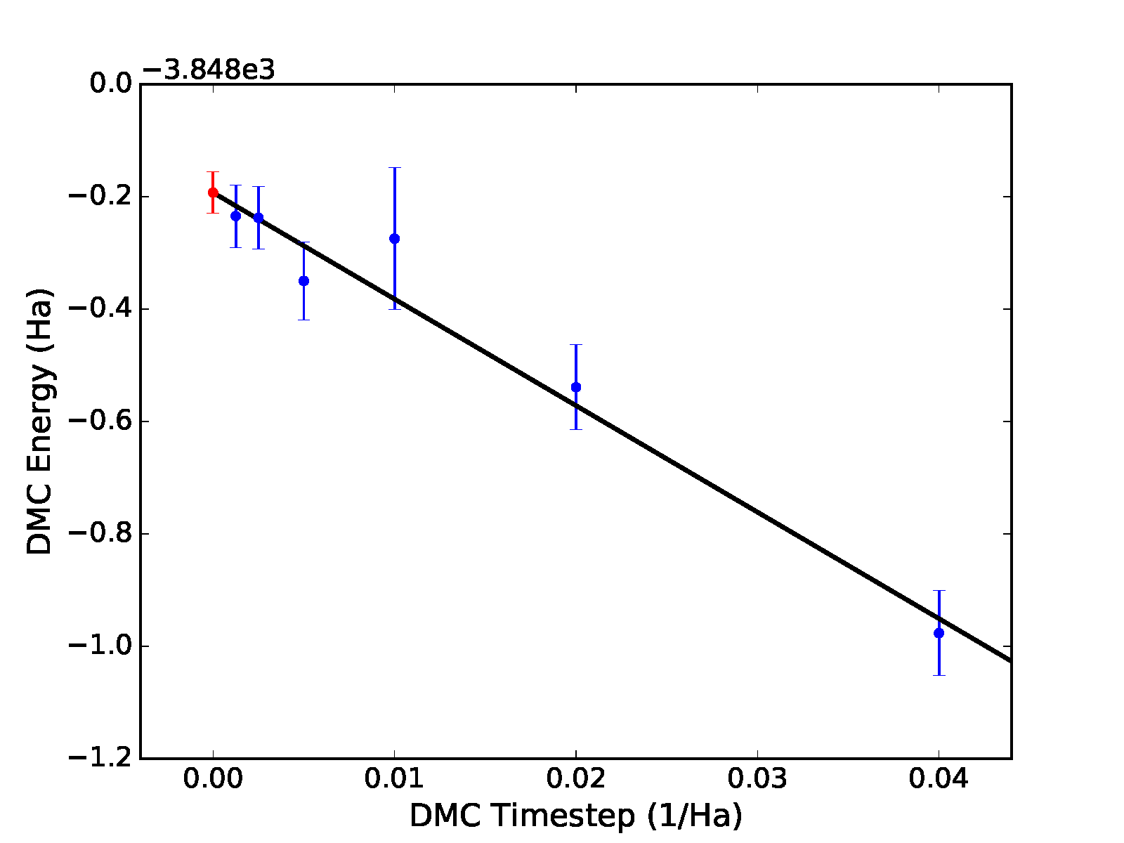
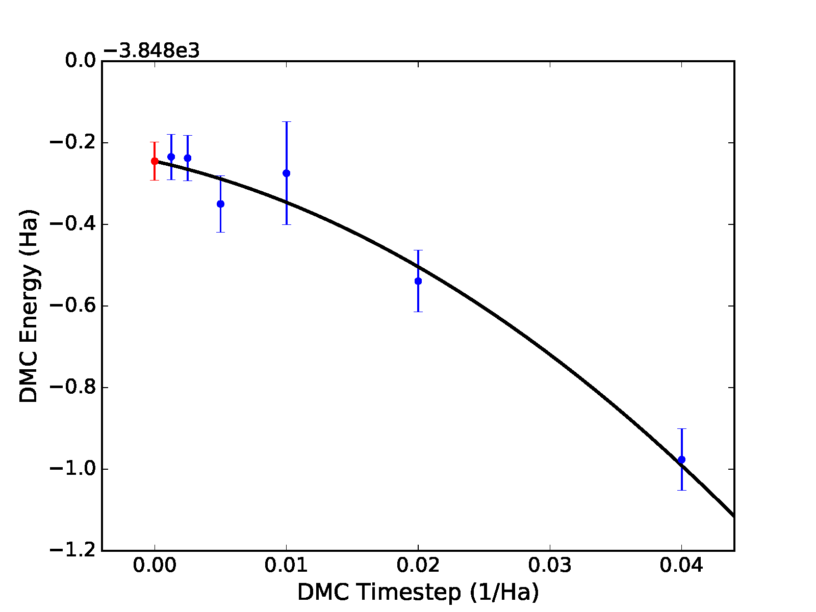
Fig. 12 Linear (top) and quadratic (bottom) time step fits to DMC data for a 32-atom supercell of MnO obtained with qmc-fit. Zero time step estimates are indicated by the red data point on the left side of either panel.
Performing trial wavefunction optimization fitting, e.g., to find optimal DFT+U
In this section, we use a 24-atom supercell of monolayer FeCl2 as an example system for wavefunction optimization
fitting. Using single determinant DFT wavefunctions, a practical method to perform wavefunction optimization is done through
scanning the Hubbard-U parameter in a DFT+U calculation used to generate the trial wavefunction. Similarly, one can also scan
different exact exchange ratio parameters in hybrid-DFT calculations. Here, we will show an example of this fitting for the
Hubbard-U parameter, but the same procedure can be applied to any single-parameter scans of trial wavefunctions. Data for this
system has been collected in DMC using the following sequence of Hubbard-U values on Fe-d orbitals: \(0 1 2 3 4 5\) eV. Some
non-zero U value often minimizes the DMC energy, but optimized U values have limited transferability across different systems.
Similar to the procedure for performing timestep statistical fitting, the quality of the input statistics must be checked using
qmca utility to determine the reblocking factor and equilibration periods. Assuming that an equilibration period of initial 50
steps, -e 50, and a reblocking period of 4, -b 6, is sufficient to remove correlations in the statistical local energies,
the qmc-fit tool can be used in the following way to obtain a quadratic fit of the data:
>qmc-fit u -e 50 -b 6 -u "0 1 2 3 4 5" -f quadratic dmc_u_*/dmc.s001.scalar.dat
fit function  : quadratic
fitted formula: (-1230.1071 +/- 0.0045) + (-0.0683 +/- 0.0040)*t + (0.00883 +/- 0.00077)*t^2
root 1 minimum_u     : 3.87 +/- 0.14 eV
root 1 minimum_e     : -1230.2391 +/- 0.0026 Ha
root 1 curvature     : 0.0177 +/- 0.0015
Here, qmc-fit u indicates we are performing a Hubbard-U/exact-exchange ratio fit,
-u option provides a list of Hubbard-U values \(0 1 2 3 4 5\) corresponding to the auto-sorted
dmc scalar files with wildcard dmc_u_*/dmc.s001.scalar.dat. Here, qmc-fit command is invoked at a
directory where folders such as dmc_u_0_2x2x1, dmc_u_1_2x2x1, dmc_u_2_2x2x1 reside.
Here, the text output provides the U value (minimum_u) and local energies (minimum_e)
at the minima of the polynomial which falls within the range of Hubbard-U values provided in the command
line, e.g. from 0 to 5. Therefore, a U value of \(3.8(1)\) eV minimizes the DMC energy of the system.
The curvature is printed for informative purposes only, but a curvature with small error bar could
indicate a higher quality polynomial fit. Similar to the timestep fit, a plot of the fit will also
produced as default where the minima of the polynomial is shown as a red dot as in Fig. 15.
Different fitting functions are supported via the -f option.
Currently supported options include quadratic (\(a+bt+ct^2\)), and
cubic (\(a+bt+ct^2+dt^3\)) and quartic (\(a+bt+ct^2+dt^3+et^4\)).
An example of a cubic fit is given as below:
>qmc-fit u -e 50 -b 6 -u "0 1 2 3 4 5" -f cubic dmc_u_*/dmc.s001.scalar.dat

fit function  : cubic
fitted formula: (-1230.1087 +/- 0.0045) + (-0.0608 +/- 0.0073)*t + (0.0047 +/- 0.0033)*t^2 + (0.00055 +/- 0.00041)*t^3
root 1 minimum_u     : 3.85 +/- 0.11 eV
root 1 minimum_e     : -1230.2415 +/- 0.0033 Ha
root 1 curvature     : 0.0221 +/- 0.0034
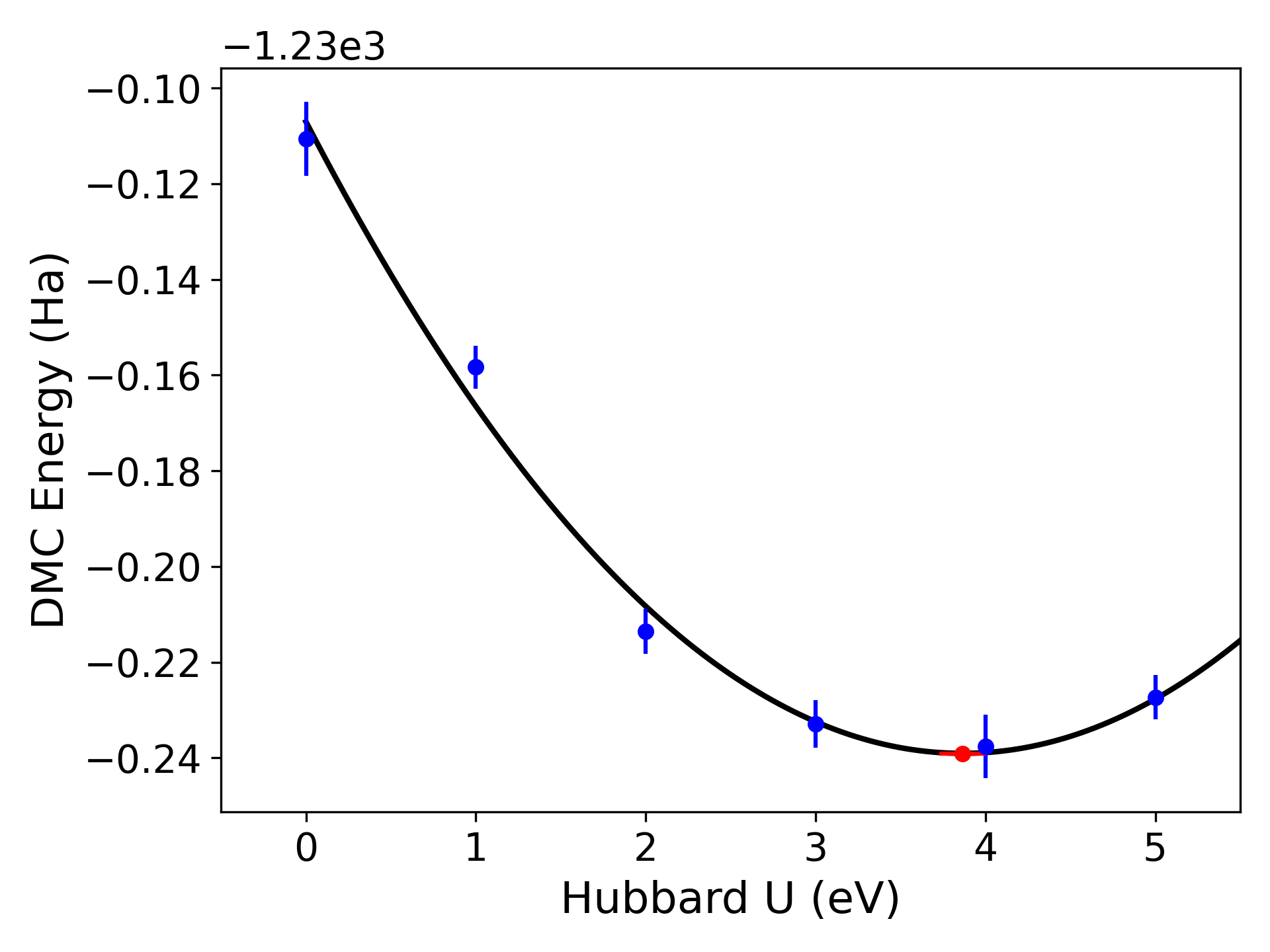
Fig. 13 Quadratic Hubbard-U fits to DMC data for a 24-atom supercell of monolayer FeCl2 obtained with qmc-fit. DMC local energy minima are indicated by the red data point on the bottom halves of either panel.
Performing equation-of-state and Morse potential binding curve fits
For a systematic series of statistical data, such as QMC calculations performed at different interatomic distances, or at a series of volumes
for an equation-of-states calculation, it is advised to perform jackknife fitting to determine quantities such as equilibrium distance, volume and
bulk moduli. For interatomic distances and equation of states fits to QMC calculations, qmc-fit has the capability to perform Morse and Birch, Murnaghan
and Vinet equation-of-state fits. In this example, we determine the equilibrium volume and bulk modulus of C-diamond using a 16 atom supercell using DMC and Murnaghan
equation-of-state fit. For the 16 atom supercell, we uniformly scan over the volumes between \(78.16\) and \(99.62 A^3\). Assuming that all these DMC calculation
folders are located under the same parent folder and ordered from smaller to the large volume (e.g. dmc_78.16, dmc_80.65 …), the following script can be used to make a
Murnaghan fit to the DMC energies.
>qmc-fit eos -e 50 -b 6 --eos "78.16 80.65 83.20 85.80 88.46 91.16 93.92 96.74 99.62" --fit murnaghan dmc_*/dmc.s001.scalar.dat

fit function  : murnaghan
fitted formula: E_inf + B/Bp*V*((V_0/V)**Bp/(Bp-1)+1)-V_0*B/(Bp-1)
minimum_x: 89.00 +/- 0.12
e_inf: -91.2659 +/- 0.0012
B: 0.1053 +/- 0.0050
Bp: 0.000189 +/- 0.000011
pressure: -0.00000 +/- 0.00015
Here, the minimum volume is reported as \(89.00 \pm 0.12A^3\) consistent with the input volume units. Considering that this is a 16-atom cell, the per atom
quantity would be \(5.56 \pm 0.01 A^3\) per C. Bulk modulus, B, is reported as \(0.1053 \pm 0.005 Ha/A^3\). In SI units, this bulk modulus value corresponds to
\(459 \pm 21\) GPa. Different fitting functions are supported via the -f option. Currently supported options include Vinet , Murnaghan, Birch and Morse.
For more information and default options, please refer to qmc-fit -h.
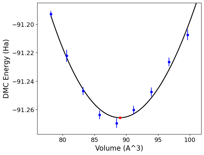
Fig. 14 Murnaghan equation-of-state fits to DMC data for a 16-atom supercell of C-diamond obtained with qmc-fit. DMC structural minimum is indicated by the red data point with an error bar smaller than its marker size.
Using the qdens tool to obtain electron densities
The qdens tool is provided to post-process the heavy density data
produced by QMCPACK and output the mean density (with and without
errorbars) in file formats viewable with, e.g., XCrysDen or VESTA. The
tool currently works only with the SpinDensity estimator in QMCPACK.
Note: this tool is provisional and may be changed or replaced at any
time. The planned successor to this tool (qstat) will expand access
to other observables and will retain at least the non-plotting
capabilities of qdens.
To use qdens, Nexus must be installed along with NumPy and H5Py. A
short list of example use cases are covered in the next section. Current
input flags are:
>qdens

Usage: qdens [options] [file(s)]

Options:
  --version             show program's version number and exit
  -h, --help            Print help information and exit (default=False).
  -v, --verbose         Print detailed information (default=False).
  -f FORMATS, --formats=FORMATS
                        Format or list of formats for density file output.
                        Options: dat, xsf, chgcar (default=None).
  -e EQUILIBRATION, --equilibration=EQUILIBRATION
                        Equilibration length in blocks (default=0).
  -r REBLOCK, --reblock=REBLOCK
                        Block coarsening factor; use estimated autocorrelation
                        length (default=None).
  -a, --average         Average over files in each series (default=False).
  -w WEIGHTS, --weights=WEIGHTS
                        List of weights for averaging (default=None).
  -i INPUT, --input=INPUT
                        QMCPACK input file containing structure and grid
                        information (default=None).
  -s STRUCTURE, --structure=STRUCTURE
                        File containing atomic structure (default=None).
  -g GRID, --grid=GRID  Density grid dimensions (default=None).
  -c CELL, --cell=CELL  Simulation cell axes (default=None).
  --density_cell=DENSITY_CELL
                        Density cell axes (default=None).
  --density_corner=DENSITY_CORNER
                        Density cell corner (default=None).
  --lineplot=LINEPLOT   Produce a line plot along the selected dimension: 0,
                        1, or 2 (default=None).
  --noplot              Do not show plots interactively (default=False).
  --twist_info=TWIST_INFO
                        Use twist weights in twist_info.dat files or not.
                        Options: "use", "ignore", "require".  "use" means use
                        when present, "ignore" means do not use, "require"
                        means must be used (default=use).
Usage examples
Process a single file, excluding the first 40 blocks, and produce XSF files:
qdens -v -e 40 -f xsf -i qmc.in.xml qmc.s000.stat.h5
Process files for all available series:
qdens -v -e 40 -f xsf -i qmc.in.xml *stat.h5
Combine groups of 10 adjacent statistical blocks together (appropriate if the estimated autocorrelation time is about 10 blocks):
qdens -v -e 40 -r 10 -f xsf -i qmc.in.xml qmc.s000.stat.h5
Apply different equilibration lengths and reblocking factors to each
series (below is appropriate if there are three series, e.g. s000,
s001, and s002):
qdens -v -e '20 20 40' -r '4 4 8' -f xsf -i qmc.in.xml *stat.h5
Produce twist averaged densities (also works with multiple series and reblocking):
qdens -v -a -e 40 -f xsf -i qmc.g000.twistnum_0.in.xml qmc.g*.s000.stat.h5
Twist averaging with arbitrary weights can be performed via the -w
option in a fashion identical to qmca.
Generate line plots of the spin-resolved twist averaged densities along the first lattice direction:
qdens -v --lineplot 0 -e 40 -a --noplot -i qmc.g000.twistnum_0.in.xml qmc.g*.s000.stat.h5
The integer supplied to --lineplot selects the axis (0 for x,
1 for y, 2 for z). Combine it with --noplot when running on
systems without a display to skip interactive windows; the plot data is
still written to disk.
Files produced
Look for files with names and extensions similar to:
qmc.s000.SpinDensity_u.xsf
qmc.s000.SpinDensity_u-err.xsf
qmc.s000.SpinDensity_u+err.xsf

qmc.s000.SpinDensity_d.xsf
qmc.s000.SpinDensity_d-err.xsf
qmc.s000.SpinDensity_d+err.xsf

qmc.s000.SpinDensity_u+d.xsf
qmc.s000.SpinDensity_u+d-err.xsf
qmc.s000.SpinDensity_u+d+err.xsf

qmc.s000.SpinDensity_u-d.xsf
qmc.s000.SpinDensity_u-d-err.xsf
qmc.s000.SpinDensity_u-d+err.xsf
Files postfixed with u relate to the up electron density, d to
down, u+d to the total charge density, and u-d to the difference
between up and down electron densities.
Files without err in the name contain only the mean, whereas files
with +err/-err in the name contain the mean plus/minus the
estimated error bar. Please use caution in interpreting the error bars
as their accuracy depends crucially on a correct estimation of the
autocorrelation time by the user (see -r option) and having a
sufficient number of blocks remaining following any reblocking.
When twist averaging, the group tag (e.g. g000 or similar) will be
replaced with avg in the names of the outputted files.
When --lineplot is requested, qdens additionally produces
.pdf and .dat files for each spin channel and derived total or
difference density. For a spin-density estimate named SpinDensity
an input file such as qmc.s000.stat.h5 yields files of the form
qmc.s000.SpinDensity_lineplot_x_u.pdf and
qmc.s000.SpinDensity_lineplot_x_u.dat (and similarly for _d,
_u+d, and _u-d). The .pdf files contain the plotted mean
densities with error bars along the chosen direction, while the matching
.dat files store the numeric coordinates and error estimates used to
create the plots.
Using the qdens-radial tool to estimate atomic occupations
Once the *Density*.xsf files are obtained from qdens, one can use the qdens-radial tool to calculate the on-site populations.
Given a set of species and radii (in Angstroms), this tool will generate a radial density – angular average – around the atomic sites up to the specified radius.
The radial density can be chosen to be non-cumulative or cumulative (integrated).
>qdens-radial

Usage: qdens-radial [options] xsf_file

Options:
  --version             show program's version number and exit
  -h, --help            Print help information and exit (default=False).
  -v, --verbose         Print detailed information (default=False).
  -r RADII, --radii=RADII
                        List of cutoff radii (default=None).
  -s SPECIES, --species=SPECIES
                        List of species (default=None).
  -a APP, --app=APP     Source that generated the .xsf file. Options: "pwscf",
                        "qmcpack" (default=qmcpack).
  -c, --cumulative      Evaluate cumulative radial density at cutoff radii
                        (default=False).
  --vmc=VMC_FILE        Location of VMC to be used for extrapolating mixed-
                        estimator bias (default=None).
  --write               Write extrapolated values to qmc-extrap.xsf
                        (default=False).
  --vmcerr=VMC_ERR_FILE
                        Location of VMC+err to be used for extrapolating
                        mixed-estimator bias and resampling (default=None).
  --dmcerr=DMC_ERR_FILE
                        Location of DMC+err to be used for resampling
                        (default=None).
  --seed=RANDOM_SEED    Random seed used for re-sampling. (default=None).
  -n NSAMPLES, --nsamples=NSAMPLES
                        Number of samples for resampling (default=50).
  -p, --plot            Show plots interactively (default=False).
Usage examples
Below are example use cases for the H2O molecule using DMC data.
Plot DMC non-cumulative radial density of the O atom:
qdens-radial -p -s O -r 1 dmc.s002.Density_q.xsf
Plot DMC cumulative radial density of the O atom:
qdens-radial -p -s O -r 1 -c dmc.s002.Density_q.xsf
For the cumulative case, qdens-radial will also print the cumulative value at the specified radius, i.e., an estimate of the atomic occupation.
Estimate of the DMC atomic occupation:
qdens-radial -p -s O -r 1.1 -c dmc.s002.Density_q.xsf
Output:
Cumulative Value of O Species at Cutoff 1.1 is: 6.55517033828574
One can also get an extrapolated estimate (mixed-estimator bias) for this quantity by providing a VMC .xsf file.
Estimate of the extrapolated atomic occupation:
qdens-radial -p -s O -r 1.1 -c --vmc=dmc.s000.Density_q.xsf dmc.s002.Density_q.xsf
Output:
Extrapolating from VMC and DMC densities...
Cumulative Value of O Species at Cutoff 1.1 is: 6.576918233167152
Error bars
One can “resample” the density at each grid point to obtain an estimate of the error bar. Recipe:
1. Use error bars from *.Density_q+err.xsf file and draw samples from a Gaussian
distribution with a standard deviation that matches the error bar.
2. Calculate occupations with resampled data and calculate standard deviation
to obtain the error bar on the occupation.
3. Make sure the number of samples (-n) is converged.
Estimate DMC atomic occupation with error bar:
qdens-radial -p -s O -r 1.1 -c -n 20 --dmcerr=dmc.s002.Density_q+err.xsf dmc.s002.Density_q.xsf
Output:
Resampling to obtain error bar (NOTE: This can be slow)...
Will compute 20 samples...
...
Cumulative Value of O Species at Cutoff 1.1 is: 6.55517033828574+/-0.001558553749396279